9 Pivoting data

This chapter explains how to use Discoverer Plus Relational's pivoting capabilities to arrange data on worksheets, and contains the following topics:

• "About pivoting worksheet items"

• "About pivoting data on a crosstab worksheet"

• "How to pivot worksheet items in the Discoverer work area"

• "How to pivot worksheet items using the Edit Worksheet dialog"

• "About unexpected results with pivoting"

9.1 About pivoting worksheet items

You pivot worksheet items to arrange data on a crosstab worksheet for more effective analysis. For example, on a crosstab worksheet you might move an item from the left axis to the top axis to analyze new data relationships.

Pivoting is a powerful analysis tool enabling you to explore data relationships that might initially be hidden.

You can pivot worksheet data in the following ways:

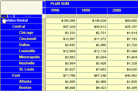
• in the Discoverer work area, you can drag and drop a worksheet item heading into a different position and see the new data layout instantly

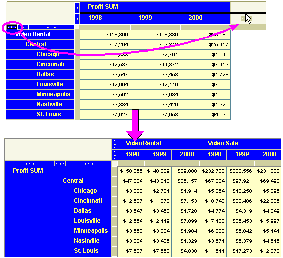
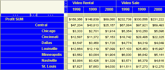
  In the example below, the Department item is dragged from the left axis to the top axis in the Discoverer work area.

  Figure 9-1 Pivoting in the Discoverer work area

  
  

  For more information about pivoting worksheet items in the Discoverer work area, see "How to pivot worksheet items in the Discoverer work area".

• in the Edit Worksheet dialog (that is, in worksheet design mode), you can drag and drop a worksheet item into a different position and see the new data layout when you close the Edit Worksheet dialog and display the Discoverer work area.

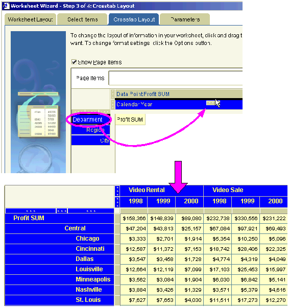
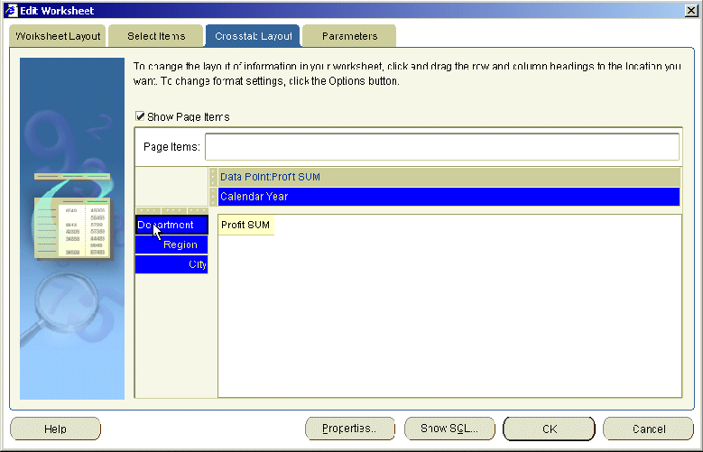
  In the example below, the Department item is dragged from the left axis to the top axis using the Edit Worksheet dialog: Table Layout tab.

  Figure 9-2 Pivoting in the Edit Worksheet dialog: Crosstab Layout tab

  
  

  For more information about pivoting worksheet items using the Edit Worksheet dialog, see "How to pivot worksheet items using the Edit Worksheet dialog".

9.2 About pivoting data on a crosstab worksheet

On crosstab worksheets, you can pivot items to and from the left axis and top axis.

Because the data relationships on a crosstab depend on the intersection of the rows and columns, pivoting data from one axis to another creates a new set of data relationships.

In addition, pivoting worksheet data can add levels of data to an axis. For example, if the data on the left axis is organized into three levels (for example, Region, City, and Store Name), pivoting the Year item to the side axis adds a fourth level of data to that axis.

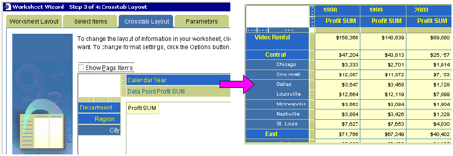
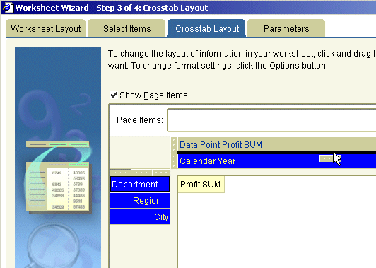
The figure below shows how you might use the Crosstab layout dialog to arrange worksheet data, by positioning items as follows:

• Calendar Year and Profit SUM items are placed on the top axis

• Department, Region, and City items are placed on the left axis

Figure 9-3 Laying out data on a crosstab worksheet

9.3 How to pivot worksheet items in the Discoverer work area

You pivot worksheet items in the Discoverer work area to rearrange items on a worksheet. For example, you might want to move a Department item to the Page Items area so that you can analyze individual departments.

To pivot worksheet items in the Discoverer work area:

1. Display the worksheet you want to analyze.

2. Select the grab handle of the worksheet item you want to pivot.

   
   

3. Drag the grab handle to the required position and release the mouse button.

   Hint: When you drag and drop items, a black line shows the item's new position on the worksheet.

   
   

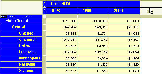
Discoverer repositions the worksheet item as you specified.

9.4 How to pivot worksheet items using the Edit Worksheet dialog

You pivot worksheet items using the Edit Worksheet dialog to rearrange items in worksheet design mode. In the Edit Worksheet dialog, you see only item headings, not the data itself. For example, you might have a large worksheet that is difficult to edit in the Discoverer work area because you cannot see all worksheet items in the same window.

To pivot worksheet items using the Edit Worksheet dialog:

1. Display the worksheet you want to analyze.

2. Choose Edit | Crosstab to display the "Edit Worksheet dialog: Crosstab Layout tab".

   
   

3. Select the name or grab handle of the item you want to pivot.

   Hint: To help you pivot items, ensure that the item labels are displayed in the Crosstab Layout tab. To display item names, choose Edit | Worksheet from the main Discoverer menu, click Properties, display the Sheet Properties tab, and select the Show item labels check box.

4. Drag the item to the required position and release the mouse button.

   Hint: When you drag and drop items, a black line shows the item's new position on the worksheet.

   
   

5. Click OK to save the details and close the Edit Worksheet dialog.

Discoverer repositions the worksheet item as you specified.

9.5 About unexpected results with pivoting

Discoverer makes it easy to pivot data on worksheets. However, it is also easy to produce unexpected results.

For example, on a crosstab worksheet, you must have the following:

• one or more items on the left axis

• one or more items on the top axis

• one or more data points (for example, Profit SUM) in the worksheet data area

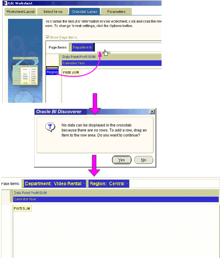
In the figure below, when the Region item on a crosstab worksheet is moved to the Page Items area, the resulting worksheet is empty. This is because you must have items on both the left axis and top axis to analyze data on a crosstab worksheet.

Figure 9-4 Pivoting to produce unexpected results