Production Scheduling Overview
This chapter covers the following topics:
Automatic Bottleneck Detection
-
Production scheduling implementation.
-
Constraint-based scheduling limitations.
-
Constraint-directed search advantages.
Production Scheduling Implementation
Production Scheduling reduces initial implementation and ongoing maintenance costs through a self-configuring solver. To understand this next-generation technology, you must consider current-generation approaches and their inherent limitations.
To implement current-generation scheduling products, you must adjust production schedules to make them usable. During this implementation adjustment phase, consultants hard-code rules for many aspects of the scheduling problem. By specifying bottlenecks, sequencing rules, and so on, you create a usable schedule. However, this approach is expensive and time consuming. Furthermore, the quality of the solution can degrade as the underlying assumptions of the hard-coded rules change. For example, changes to demand mix and capacity constraints are normal in any business, but they change the assumptions of the original rules and, subsequently, reduce the quality of the schedule. As schedule quality degrades, planners try to maintain quality by overriding the system with time consuming and subjective manual schedule changes. Planners often stop using the system entirely and revert to their previous planning methods.
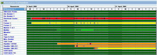
Production Scheduling provides the ability to detect resource bottlenecks automatically, even when they dynamically float, or move, within a given schedule. Resource bottlenecks may float from crew to tool, and then to materials, to machine, and so on throughout the scheduling horizon. Using knowledge about resource bottlenecks, the Production Scheduling solver employs a scheduling strategy that exploits each type of bottleneck and maximizes manufacturing throughput. As a result, no initial rule configuration and schedule quality remains consistent over the life cycle of the implementation. Instead of focusing on customizing and maintaining rules, the planner can focus on scheduling. Dynamic bottleneck detection is such an important concept in Production Scheduling that a specific view is dedicated to the visualization of bottlenecks while schedules are being solved. The Resource Contention view enables planners to watch the Production Scheduling solver dynamically detect and exploit resource bottlenecks. Red indicates serious resource criticality. Shades of orange, yellow, and green indicate decreasing criticality, with green indicating the least criticality. Once the solve finishes, the Resource Contention view displays a histogram of the resources that drove the majority of scheduling decisions.
For example, in this example, the planner can see that the red Electrical Tester machine is the dominant resource bottleneck at that point in the solve:
The technology that enables users to detect bottlenecks automatically is called Constraint Directed Search (CDS). CDS is the logical evolution of constraint-based scheduling, but it does not have the limitations that historically affected constraint-based approaches.
Constraint-Based Scheduling Limitations
Constraint-based schedules provide an accurate and detailed model of the factory. Constraint propagation is also an efficient method for determining the consequences of scheduling decisions. However, although propagation usually finds a feasible solution, it often requires an excessive amount of time, particularly for large problems. These large problems are relatively common; therefore, the application of this technology in the real world has been slow because:
-
A constraint-based scheduler must assign a start time to each operation and resolve resulting conflicts before a feasible solution can be reached.
This delay causes the system to move data around rather than performing useful computation (known as thrashing ) and leads to backtracking (undoing unworkable decisions), which significantly increases the time needed to find a solution.
-
To prevent thrashing, implementation personnel must customize algorithms for each implementation.
Because this approach takes an existing set of rules and tries to fit those rules to a new problem, the algorithm requires numerous adjustments. These adjustments often require changes to the application source code, which compromises future upgrades and increases the time and cost of the implementation. In addition, custom algorithms cannot respond satisfactorily to automatic floating bottleneck detection.
-
As a result of customization, current-generation technology is not generally applicable.
If business requirements change, the technology cannot respond without further customization, delays, and expense.
-
In many cases, current generation solvers cannot find good solutions even when they exist.
Constraint Directed Search Advantages
Constraint Directed Search (CDS) provides the advantages of constraint-based scheduling without the disadvantages of performance problems. This improved technology, which reduces guesswork and prevents wrong decisions, uses:
-
Texture measurements to:
-
Determine which decision is most critical by measuring local schedule conditions, which identify bottlenecks before a decision is made.
-
Minimize or eliminate backtracking by returning to the last decision made or to the most uncertain decision that was previously made.
-
Allow larger problems to be solved.
-
Reduce solve time.
-
-
Least commitment to:
-
Assign operation precedence constraints so that a start time does not need to be assigned.
These constraints allow operations to float within a time range until the end, when an explicit start time is assigned.
-
Find the critical paths in a schedule.
-
Allow scheduling flexibility by tracking slack time.
-
Avoid deadlocks in the propagation process.
-
Optimize start time after sequencing.
-
Allow dynamic schedule monitoring, for example, to determine whether a late starting operation will cause the order to be late.
-
The Production Scheduling application supports both generative scheduling and repair-based scheduling. Production Scheduling allows forward and backward propagation as well as propagation in all dimensions of a scheduling problem, including resource utilization and inventory.
Advanced Analytical Decision Support
-
Production Pegging view.
-
Resource Gantt and Resource Utilization combined view.
-
Resource Gantt and Operation Gantt combined view.
-
Resource Gantt, Operation Gantt, and Item Graph combined view.
Note: The views listed are only a subset of the analytical views that the Production Scheduling application supports. The eight basic views can be used on their own or combined through the use of a Wizard.
Production Pegging View
From Production Scheduling, you can analyze your schedule in various views. The Production Pegging view is used to analyze projected customer service levels and the supply constraints that dictate those levels. All purchased and manufactured supply is pegged to a demand line item. This view can identify which orders are late and what specific condition is preventing these orders from being on time.
The Production Pegging view supports these key capabilities:
-
User-defined demand sorting.
-
Graphical-demand fill rates.
-
Exceptions with suggested root cause.
-
Dynamic-demand filtering.
User-Defined Demand Sorting
Demand sorting (for sales orders, forecasts, and so on) is defined by a user-defined folder structure, which is specified in the Supply & Demand Editor. The folder structure can represent product types, demand types, customer hierarchies, and so on, and it provides an intuitive structure for analyzing the schedule.
Graphical-Demand Fill Rates
The folder summary bars have various colors that indicate the amount of on-time demand or the unit fill percent. Demands or demand folders with red summary bars indicate less than 33 percent of on-time units, orange summary bars indicate between 33 and 66 percent of on-time units, yellow summary bars indicate between 66 and 99 percent of on-time units, and black summary bars indicate 100 percent of on-time units. Position your cursor over a summary bar to see a description of the fill rate and details about late demand.
Exceptions with Suggested Root Cause
When a schedule is solved, Production Scheduling analyzes the results, identifies potential problems and their possible root cause, and generates the appropriate exceptions. Production Scheduling supports a variety of exceptions. One exception type alerts you to projected late orders and their suggested root causes. From the exception message, you can access the Production Pegging view, which automatically opens the Production Pegging view tree to the bottleneck operation that is pegged to the late demand.
Dynamic-Demand Filtering
You can filter thousands of orders by user-specific criteria, which, in turn, enables you to manage by exception. For example, if eight of 31 line items occur late in a schedule, then you can filter the lines that are less than one day late. By filtering, you can learn that only four line items are more than one day late. All other orders are temporarily filtered out.
Resource Gantt and Resource Utilization Combined View
This view displays the details of scheduled operations on their machines, crews, and tools, while viewing resource utilization for the currently selected resource in a bar chart. This view displays utilization by shift, daily, weekly, or monthly buckets. By selecting a particular time bucket, you can view the breakdown of idle, delay, down, changeover, and run time.
The Resource Utilization view also displays utilization across groups of resources. This view is useful to identify the aggregate utilization of like resources, such as a pool of machines or crew.
Resource Gantt and Operation Gantt Combined View
This view displays how operations are scheduled. All operations for the selected resource appear in the lower pane, sorted chronologically.
Automatic sorting occurs based on the context of the zoom at the moment the resource is selected. Therefore, when zooming in or out, you can reselect the resource to re-sort the operations.
Resource Gantt, Operation Gantt and Item Graph Combined View
Although the Production Pegging view is ideal for a Make-to-Order (MTO) environment, the Resource Gantt, Operation Gantt and Item Graph combined view is ideal for a Make-to-Stock (MTS) environment. Examples of Make-to-Stock environments are Consumer Packaged Goods, and Food and Beverage.
The Resource Gantt and Operation Gantt panes in this view display the sequence being run on each resource. In the previous example, you can see that Packer 1 has a weekly campaign cycle for which time lost to sequence-dependent changeovers has been minimized. When you select each packing operation, the Item Graph pane displays the produced and consumed inventory levels, and inventory levels are perfectly supported.
Direct Scenario Comparisons
Production Scheduling can compare different schedule scenarios. During one session, a planner can create an unlimited number of scenarios and then compare them using the Key Performance Indicators (KPI) view.
The system provides standard supply chain metrics to assess which scenario best meets your business objectives. Scenarios can be sorted by the Key Performance Indicators of interest and evaluated to identify the best possible schedule solution. Conversely, most competitive products support only a single scenario in one session, which forces planners to repeatedly save the various scenarios and run multiple sessions simultaneously, making the ideal scenario difficult to determine. In addition to KPI comparisons, schedules can be directly compared to each other from a customer service perspective, allowing you to understand which scenario best meets customer service objectives. Scenario comparison can help answer the following questions:
-
In this new scenario, which work orders or demands are now on time compared to my best scenario previously?
-
In this new scenario, which work orders or demands are now late compared to my best scenario previously?
-
In this new scenario, what is the effect on overall earliness or lateness?
After a planner decides which schedule they prefer, they approve it and then publish it to a resource planning application.