3.5.1 Amdahl’s Law

Fixed problem-size speedup is generally governed by Amdahl’s law. Amdahl’s Law simply says that the amount of parallel speedup in a given problem is limited by the sequential portion of the problem.The following equation describes the speedup of a problem where F is the fraction of time spent in sequential region, and the remaining fraction of the time is spent uniformly among P processors. If the second term of the equation drops to zero, the total speedup is bounded by the first term, which remains fixed.

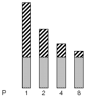
The following figure illustrates this concept diagrammatically. The darkly shaded portion represents the sequential part of the program, and remains constant for one, two, four, and eight processors, while the lightly shaded portion represents the parallel portion of the program that can be divided uniformly among an arbitrary number of processors.

Figure 3–3 Fixed Problem Speedups

As the number of processors increases, the amount of time required for the parallel portion of each program decreases whereas the serial portion of each program stays the same.

In reality, however, you may incur overheads due to communication and distribution of work to multiple processors. These overheads may or may not be fixed for arbitrary number of processors used.

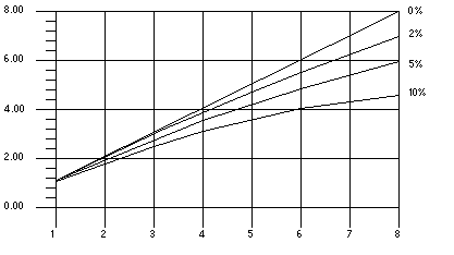
The following figure illustrates the ideal speedups for a program containing 0%, 2%, 5%, and 10% sequential portions. Here, no overhead is assumed.

Figure 3–4 Amdahl's Law Speedup Curve

A graph that shows the ideal speedups for a program containing 0%, 2%, 5%, and 10% sequential portions, assuming no overhead. The x-axis measures the number of processors and the y-axis measures the speedup.

3.5.1.1 Overheads

Once the overheads are incorporated in the model the speedup curves change dramatically. Just for the purposes of illustration we assume that overheads consist of two parts: a fixed part which is independent of the number of processors, and a non-fixed part that grows quadratically with the number of the processors used:

The fraction one over S equals one divided by the quantity of F plus the quantity one minus the fraction F over P end of quantity plus K sub one plus K sub two times P squared end quantity.

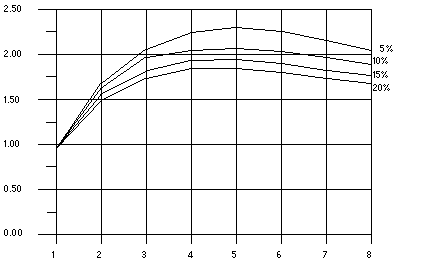
In this equation, K₁ and K₂ are some fixed factors. Under these assumptions the speedup curve is shown in the following figure. It is interesting to note that in this case the speedups peak out. After a certain point adding more processors is detrimental to performance as shown in the following figure.

Figure 3–5 Speedup Curve With Overheads

The graph shows that all programs reach the greatest speedup at five processors and then loose this benefit as up to eight processors are added. The x-axis measures the number of processors and the y-axis measures the speedup.

3.5.1.2 Gustafson’s Law

Amdahls Law can be misleading for predicting parallel speedups in real problems. The fraction of time spent in sequential sections of the program sometimes depends on the problem size. That is, by scaling the problem size, you may improve the chances of speedup. The following example demonstrates this.

Example 3–12 Scaling the Problem Size May Improve Chances of Speedup

/*
* initialize the arrays
*/
for (i=0; i < n; i++) {
    for (j=0; j < n; j++) {
            a[i][j] = 0.0;
            b[i][j] = ...
            c[i][j] = ...
    }
}
/*
* matrix multiply
*/
for (i=0; i < n; i++) {
    for(j=0; j < n; j++) {
            for (k=0; k < n; k++) {
                a[i][j] = b[i][k]*c[k][j];
            }
    }
}

Assume an ideal overhead of zero and assume that only the second loop nest is executed in parallel. It is easy to see that for small problem sizes (i.e. small values of n), the sequential and parallel parts of the program are not so far from each other. However, as n grows larger, the time spent in the parallel part of the program grows faster than the time spent in the sequential part. For this problem, it is beneficial to increase the number of processors as the problem size increases.