Using conditional formatting in Discoverer

Conditional formatting is the use of conditional formats and stoplight formats to highlight worksheet values. This section explains how use conditional formatting in Discoverer Viewer, and contains the following topics:

"What is a conditional format?"
"What is a stoplight format?"
"How to activate and deactivate conditional formats"
"How to create a conditional format"
"How to create a stoplight format"
"How to create a stoplight format"
"How to create a conditional header format"
"How to edit conditional formats"
"How to delete conditional formats"

What is a conditional format?

A conditional format enables you to highlight worksheet values that meet a specific condition. For example, you might want to highlight profit values greater than 30,000.

Note: In Discoverer Desktop, conditional formats are known as exceptions.

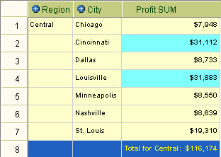
In the example below, a conditional format highlights Profit SUM values greater than 30,000. The Profit SUM figures for Cincinnati and Louisville are displayed with a blue background because they are greater than 30,000.

Figure 3-1 A Discoverer worksheet using a conditional format

Description of the illustration d_cf1.gif

What is a stoplight format?

A stoplight format (or traffic light format) enables you to categorize numeric worksheet values as unacceptable, acceptable, and desirable using different colors. The default stoplight format uses the familiar red, yellow, and green color scheme to represent unacceptable, acceptable, and desirable values.

For example, you might want to categorize performance based on profit values where:

values less than or equal to 10,000 are unacceptable, and are shown in red
values between 10,001 and 29,999 are acceptable, and are shown in yellow
values equal to or greater than 30,000 are desirable, and are shown in green

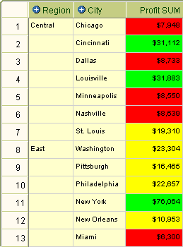
In the example below, a stoplight format based on the above values is used to categorize Profit SUM values. Values in the unacceptable category are show in red (e.g. Chicago and Dallas). Values in the acceptable category are shown in yellow (e.g. St. Louis and Washington). Values in the desirable category are shown in green (e.g. Cincinnati and Louisville).

Figure 3-2 A Discoverer worksheet using a stoplight format

Description of the illustration d_cf2.gif

What is a conditional header format?

A conditional header format enables you to change the appearance of selected worksheet item headings. For example, you might want to display the heading for items Year and Region with a blue background, leaving the items Profit SUM with the default white background.

How to activate and deactivate conditional formats

You activate a conditional format to apply that format to the currently displayed worksheet. For example, you might want to use an existing conditional format to highlight percentage values greater than 75% by displaying them with a blue background.

You deactivate a conditional format to remove that format from the currently displayed worksheet. For example, you might want to remove a conditional format that highlights percentage values greater than 75% by displaying them with a blue background. You can always activate the conditional format later.

For more information, see "What is a conditional format?".

To activate and deactivate a conditional format:

Display the worksheet that you want to analyze (for more information, see "How to open a Discoverer worksheet").
Select the Format link to display formatting tools above the worksheet data.
Select the Conditional Formats link to display the "Conditional Formats (Table/Crosstab) page".
To activate a conditional format, select the check box in the Display column next to the format you want to activate.
To deactivate a conditional format, clear the check box in the Display column next to the format you want to deactivate.
Click Apply to save the changes and display the worksheet.

Discoverer applies the format changes you have specified.

Hint: Select the minus (-) icon next to the Tools label to hide the formatting tools.

How to change the precedence of conditional format

When two formats specify different settings for the same cell, the most recently created format takes precedence. For example, when you set the background color for a column to blue, and then set the background color for a row to red, the intersecting cell has a red background.

The order of the formats in the Conditional Formats <Crosstab | Table> page determines which format applies in the case of a conflict. The higher format in the list takes precedence over lower formats.

For more information, see "What is a conditional format?".

To change the precedence of a conditional format:

Display the worksheet that you want to analyze (for more information, see "How to open a Discoverer worksheet").
Select the Format link to display formatting tools above the worksheet data.
Select the Conditional Formats link to display the "Conditional Formats (Table/Crosstab) page".
Click the Move Up icon next to the conditional format that you want to apply.
Click Apply to save the changes and display the worksheet.

Discoverer applies the format changes you have specified.

Hint: Select the minus (-) icon next to the Tools label to hide the formatting tools.

How to create a conditional format

You create a conditional format to highlight worksheet values that meet a specific condition. For example, you might want to highlight percentage values greater than 75% by displaying them with a blue background.

For more information, see "What is a conditional format?".

Note: To categorize worksheet values as unacceptable, acceptable, and desirable using color and text formatting, you create a stoplight format and not a conditional format (for more information, see "How to create a stoplight format").

To create a conditional format?

Display the worksheet that you want to analyze (for more information, see "How to open a Discoverer worksheet").
Select the Format link to display formatting tools above the worksheet data.
Select the Create Conditional Format link to display the "Create Conditional Cell Format page".
Use the "Create Conditional Cell Format page" to select the worksheet item that you want to format, and specify format colors and styles.
Click Apply to save the changes and display the worksheet.

Discoverer applies the format changes you have specified.

Hint: Select the minus (-) icon next to the Tools label to hide the formatting tools.

How to create a stoplight format

You create a stoplight format when you want to categorize numeric worksheet values as unacceptable, acceptable, and desirable using text and color formatting. For example, you might want to display low cost values in green, medium cost values in yellow, and high cost values in red.

For more information, see "What is a stoplight format?".

To create a stoplight format?

Display the worksheet that you want to analyze (for more information, see "How to open a Discoverer worksheet").
Select the Stoplight link to display stoplight formatting tools above the worksheet data.
Use the Format drop down list to specify whether to apply the format to all cells, selected cells, or to cells for an item or measure.
Enter threshold values in the Unacceptable and Desirable fields.

Note: Threshold values are inclusive. For example, if you select 30,000 in the Desirable field, you apply this category to value equal to or greater than 30,000.
(optional) Select the color palette icons next to the Unacceptable, Acceptable, and Desirable fields to display a color palette and change the color for that category.
Click Go to apply the stoplight format to the worksheet.

Discoverer applies the format changes you have specified.

Hint: Select the minus (-) icon next to the Tools label to hide the formatting tools.

How to create a conditional header format

You create a conditional header format to change the look and feel of particular worksheet item headings. For example, you might want to change the background color of the worksheet item header for a Region item to blue.

For more information, see "What is a conditional header format?".

To create a conditional header format:

Display the worksheet that you want to analyze (for more information, see "How to open a Discoverer worksheet").
Select the Format link to display stoplight formatting tools above the worksheet data.
Select the Conditional Formats link to display the "Conditional Formats (Table/Crosstab) page".
Click Create Conditional Header Format to display the "How to create a conditional header format".
Use the "Create Conditional Header Format page" to select the worksheet item that you want to format, and specify format colors and styles.
Click Apply to save the changes and display the "Conditional Formats (Table/Crosstab) page".
Click Apply to close the "Conditional Formats (Table/Crosstab) page" and display the worksheet.

Discoverer applies the format changes you have specified.

Hint: Select the minus (-) icon next to the Tools label to hide the formatting tools.

How to edit conditional formats

You edit a conditional format to change how it works. For example, you might want to change the color of the Acceptable stoplight category from yellow to orange.

To edit a conditional format:

Display the worksheet that you want to analyze (for more information, see "How to open a Discoverer worksheet").
Select the Format link to display formatting tools above the worksheet data.
Select the Conditional Formats link to display the "Conditional Formats (Table/Crosstab) page".
Select the pencil icon in the Edit column next to the format you want to change to display the edit page for that type of format.
Make the necessary changes to the formats.
Click Apply to save the changes and close the edit page.
Click Apply to close the "Conditional Formats (Table/Crosstab) page" and display the worksheet.

Discoverer applies the format changes you have specified.

Hint: Select the minus (-) icon next to the Tools label to hide the formatting tools.

How to delete conditional formats

You delete a conditional format to remove it permanently from the currently displayed worksheet. For example, you might want to delete a conditional format that highlights percentage values greater than 75% by displaying them with a blue background.

Hint: If you think you might want to use the conditional format again, consider deactivating the conditional format rather than deleting it (for more information, see "How to activate and deactivate conditional formats").

To delete a conditional format:

Display the worksheet that you want to analyze (for more information, see "How to open a Discoverer worksheet").
Select the Format link to display formatting tools above the worksheet data.
Select the Conditional Formats link to display the "Conditional Formats (Table/Crosstab) page".
Select the trash can icon in the Delete column next to the conditional format you want to delete.

Hint: To remove all formatting applied using the Formatting toolbar from the current worksheet, click Clear All Formatting, and click Yes at the confirmation page.
Click Apply to save the changes and display the worksheet.

Discoverer applies the format changes you have specified.

Hint: Select the minus (-) icon next to the Tools label to hide the formatting tools.