4 Regression

This chapter describes regression, the supervised mining function for predicting a continuous, numerical target.

About Regression

Regression is a data mining function that predicts a number. Profit, sales, mortgage rates, house values, square footage, temperature, or distance could all be predicted using regression techniques. For example, a regression model could be used to predict the value of a house based on location, number of rooms, lot size, and other factors.

A regression task begins with a data set in which the target values are known. For example, a regression model that predicts house values could be developed based on observed data for many houses over a period of time. In addition to the value, the data might track the age of the house, square footage, number of rooms, taxes, school district, proximity to shopping centers, and so on. House value would be the target, the other attributes would be the predictors, and the data for each house would constitute a case.

In the model build (training) process, a regression algorithm estimates the value of the target as a function of the predictors for each case in the build data. These relationships between predictors and target are summarized in a model, which can then be applied to a different data set in which the target values are unknown.

Regression models are tested by computing various statistics that measure the difference between the predicted values and the expected values. The historical data for a regression project is typically divided into two data sets: one for building the model, the other for testing the model. See "Testing a Regression Model".

Regression modeling has many applications in trend analysis, business planning, marketing, financial forecasting, time series prediction, biomedical and drug response modeling, and environmental modeling.

How Does Regression Work?

You do not need to understand the mathematics used in regression analysis to develop and use quality regression models for data mining. However, it is helpful to understand a few basic concepts.

Regression analysis seeks to determine the values of parameters for a function that cause the function to best fit a set of data observations that you provide. The following equation expresses these relationships in symbols. It shows that regression is the process of estimating the value of a continuous target (y) as a function (F) of one or more predictors (x₁ , x₂ , ..., x_n), a set of parameters (θ₁ , θ₂ , ..., θ_n), and a measure of error (e).

y = F(x,θ)  + e

The predictors can be understood as independent variables and the target as a dependent variable. The error, also called the residual, is the difference between the expected and predicted value of the dependent variable. The regression parameters are also known as regression coefficients. (See "Regression Coefficients".)

The process of training a regression model involves finding the parameter values that minimize a measure of the error, for example, the sum of squared errors.

There are different families of regression functions and different ways of measuring the error.

Linear Regression

A linear regression technique can be used if the relationship between the predictors and the target can be approximated with a straight line.

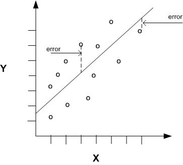
Regression with a single predictor is the easiest to visualize. Simple linear regression with a single predictor is shown in Figure 4-1.

Figure 4-1 Linear Regression With a Single Predictor

Description of "Figure 4-1 Linear Regression With a Single Predictor"

Linear regression with a single predictor can be expressed with the following equation.

y = θ2x   +  θ1  + e

The regression parameters in simple linear regression are:

The slope of the line (θ₂) — the angle between a data point and the regression line
The y intercept (θ₁) — the point where x crosses the y axis (x = 0)

Multivariate Linear Regression

The term multivariate linear regression refers to linear regression with two or more predictors (x₁, x₂, …, x_n). When multiple predictors are used, the regression line cannot be visualized in two-dimensional space. However, the line can be computed simply by expanding the equation for single-predictor linear regression to include the parameters for each of the predictors.

y = θ1 +  θ2x1  +  θ3x2   + .....  θn  xn-1  + e

Regression Coefficients

In multivariate linear regression, the regression parameters are often referred to as coefficients. When you build a multivariate linear regression model, the algorithm computes a coefficient for each of the predictors used by the model. The coefficient is a measure of the impact of the predictor x on the target y. Numerous statistics are available for analyzing the regression coefficients to evaluate how well the regression line fits the data. ("Regression Statistics".)

Nonlinear Regression

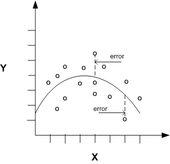
Often the relationship between x and y cannot be approximated with a straight line. In this case, a nonlinear regression technique may be used. Alternatively, the data could be preprocessed to make the relationship linear.

Nonlinear regression models define y as a function of x using an equation that is more complicated than the linear regression equation. In Figure 4-2, x and y have a nonlinear relationship.

Figure 4-2 Nonlinear Regression With a SIngle Predictor

Description of "Figure 4-2 Nonlinear Regression With a SIngle Predictor"

Multivariate Nonlinear Regression

The term multivariate nonlinear regression refers to nonlinear regression with two or more predictors (x₁, x₂, …, x_n). When multiple predictors are used, the nonlinear relationship cannot be visualized in two-dimensional space.

Confidence Bounds

A regression model predicts a numeric target value for each case in the scoring data. In addition to the predictions, some regression algorithms can identify confidence bounds, which are the upper and lower boundaries of an interval in which the predicted value is likely to lie.

When a model is built to make predictions with a given confidence, the confidence interval will be produced along with the predictions. For example, a model might predict the value of a house to be $500,000 with a 95% confidence that the value will be between $475,000 and $525,000.

A Sample Regression Problem

Suppose you want to learn more about the purchasing behavior of customers of different ages. You could build a model to predict the ages of customers as a function of various demographic characteristics and shopping patterns. Since the model will predict a number (age), we will use a regression algorithm.

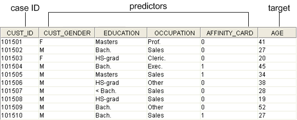
This example uses the regression model, svmr_sh_regr_sample, which is created by one of the Oracle Data Mining sample programs. Figure 4-3 shows six columns and ten rows from the case table used to build the model. The affinity_card column can contain either a 1, indicating frequent use of a preferred-buyer card, or a 0, which indicates no use or infrequent use.

Figure 4-3 Sample Build Data for Regression

Description of "Figure 4-3 Sample Build Data for Regression"

After undergoing testing (see "Testing a Regression Model"), the model can be applied to the data set that you wish to mine.

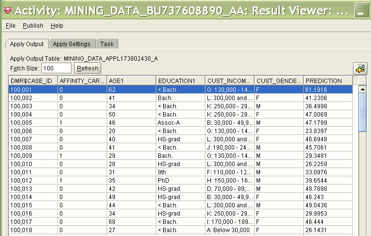
Figure 4-4 shows some of the predictions generated when the model is applied to the customer data set provided with the Oracle Data Mining sample programs. Several of the predictors are displayed along with the predicted age for each customer.

Figure 4-4 Regression Results in Oracle Data Miner

Description of "Figure 4-4 Regression Results in Oracle Data Miner"

Note:

Oracle Data Miner displays the generalized case ID in the DMR$CASE_ID column of the apply output table. A "1" is appended to the column name of each predictor that you choose to include in the output. The predictions (the predicted ages in Figure 4-4) are displayed in the PREDICTION column.

Testing a Regression Model

A regression model is tested by applying it to test data with known target values and comparing the predicted values with the known values.

The test data must be compatible with the data used to build the model and must be prepared in the same way that the build data was prepared. Typically the build data and test data come from the same historical data set. A percentage of the records is used to build the model; the remaining records are used to test the model.

Test metrics are used to assess how accurately the model predicts these known values. If the model performs well and meets the business requirements, it can then be applied to new data to predict the future.

Residual Plot

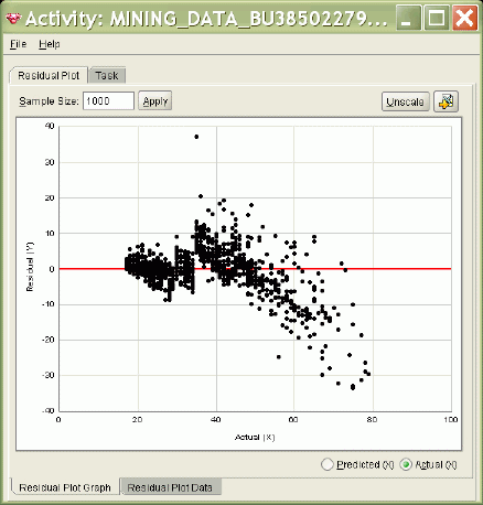
A residual plot is a scatter plot where the x-axis is the predicted value of x, and the y-axis is the residual for x. The residual is the difference between the actual value of x and the predicted value of x.

Figure 4-5 shows a residual plot for the regression results shown in Figure 4-4. Note that most of the data points are clustered around 0, indicating small residuals. However, the distance between the data points and 0 increases with the value of x, indicating that the model has greater error for people of higher ages.

Figure 4-5 Residual Plot in Oracle Data Miner

Description of "Figure 4-5 Residual Plot in Oracle Data Miner"

Regression Statistics

The Root Mean Squared Error and the Mean Absolute Error are commonly used statistics for evaluating the overall quality of a regression model. Different statistics may also be available depending on the regression methods used by the algorithm.

Root Mean Squared Error

The Root Mean Squared Error (RMSE) is the square root of the average squared distance of a data point from the fitted line.

This SQL expression calculates the RMSE.

SQRT(AVG((predicted_value - actual_value) * (predicted_value - actual_value)))

This formula shows the RMSE in mathematical symbols. The large sigma character represents summation; j represents the current predictor, and n represents the number of predictors.

Description of the illustration rmse.gif

Mean Absolute Error

The Mean Absolute Error (MAE) is the average of the absolute value of the residuals (error). The MAE is very similar to the RMSE but is less sensitive to large errors.

This SQL expression calculates the MAE.

AVG(ABS(predicted_value - actual_value))

This formula shows the MAE in mathematical symbols. The large sigma character represents summation; j represents the current predictor, and n represents the number of predictors.

Description of the illustration mae.gif

Test Metrics in Oracle Data Miner

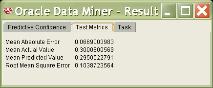
Oracle Data Miner calculates the regression test metrics shown in Figure 4-6.

Figure 4-6 Test Metrics for a Regression Model

Description of "Figure 4-6 Test Metrics for a Regression Model"

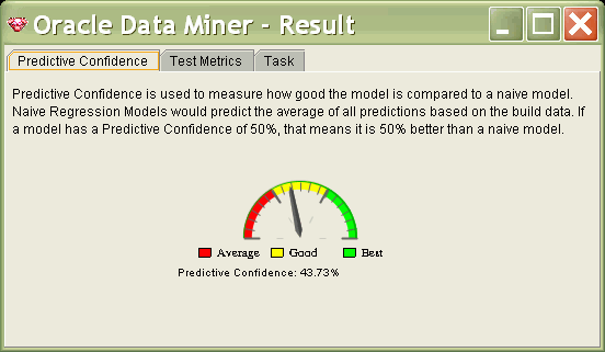
Oracle Data Miner calculates the predictive confidence for regression models. Predictive confidence is a measure of the improvement gained by the model over chance. If the model were "naive" and performed no analysis, it would simply predict the average. Predictive confidence is the percentage increase gained by the model over a naive model. Figure 4-7 shows a predictive confidence of 43%, indicating that the model is 43% better than a naive model.

Figure 4-7 Predictive Confidence for a Regression Model

Description of "Figure 4-7 Predictive Confidence for a Regression Model"

Regression Algorithms

Oracle Data Mining supports two algorithms for regression. Both algorithms are particularly suited for mining data sets that have very high dimensionality (many attributes), including transactional and unstructured data.

Generalized Linear Models (GLM)

GLM is a popular statistical technique for linear modeling. Oracle Data Mining implements GLM for regression and for binary classification.

GLM provides extensive coefficient statistics and model statistics, as well as row diagnostics. GLM also supports confidence bounds.
Support Vector Machines (SVM)

SVM is a powerful, state-of-the-art algorithm for linear and nonlinear regression. Oracle Data Mining implements SVM for regression and other mining functions.

SVM regression supports two kernels: the Gaussian kernel for nonlinear regression, and the linear kernel for linear regression. SVM also supports active learning.