Engine Details

This chapter provides details on the Analytical Engine, for the benefit of advanced users.

This chapter covers the following topics:

• Preparing the Database
• Promotion Effectiveness Engine Phases
• The Forecasting Process
• Comparison of Batch and Simulation Modes
• Engine Components and High-Level Flow
• Details of the Distributed Engine

Preparing the Database

At the start of an engine run, the Analytical Engine prepares the database, to make sure that the appropriate tables contain rows into which the Analytical Engine can write results. To do so, the Analytical Engine calls the INSERT_UNITS procedure, which is controlled by the RunInsertUnits parameter and can do several things, depending on the value of that parameter:

• Makes sure the engine has rows to write into when generating the forecast. In particular, for all non-dead combinations, this procedure does the following:

  1. Checks to see if the database contains records for this combination for all dates in the span of time from max_sales_date to max_sales_date + lead.

  2. For any dates when the combination does not have records, this procedure inserts records with zero sales, into which the Analytical Engine can then write the forecast.

  3. Records with dates in the past are ignored.

• Runs the EXECUTE_PROFILES procedure, which executes the active rolling data profiles.

Additional Details for PE Mode

For Promotion Effectiveness, if the DeleteIsSelfRows parameter is 1, the Analytical Engine also performs a cleaning step. In this step, it removes unneeded rows from the promotion_data, which otherwise can grow to an unreasonable size. (If this table contained a row for every item, every location, every promotion, and every date, performance would suffer.) Specifically, the Analytical Engine deletes rows that have is_self is 0 and that have zero lift values (details below).

In some cases, users may enter override values, and the Analytical Engine should not delete rows that contain those values. The DeleteIsSelfCondition parameter specifies other fields in promotion_data that should be checked before this cleaning occurs. The Analytical Engine deletes only the rows that have is_self is 0 and zero values for all of the following fields: uplift, pre and post-effect, switching effects, and the field or fields specified by DeleteIsSelfCondition.

Promotion Effectiveness Engine Phases

In PE mode, the Analytical Engine runs in multiple phases (the last of which actually generates the forecast), and it caches data at critical points, for better performance. The earlier phases map the promotion attributes internally into causal factors, so that they can be used in the same way as the other causal factors.

This section describes these engine phases.

Global Preparations

This phase uses the following settings from the Promotional Causal Factor screen; see "Configuring Promotional Causal Factors":

Column Name Expression	An expression that retrieves and aggregates the promotion attribute.
Filter	An aggregating expression that returns the true or false value, filtering the source data of this promotional causal factor. You can use this expression to create multiple causal factors from a single set of source data.

When the Analytical Engine runs, the first step is to perform the following global preparations:

• Create the promotion_data_engine table, which is analogous to the sales_data_engine used in demand planning.

• In memory, aggregate the promotion attribute data to the lowest promotional level, as defined in the forecast tree. Here the Analytical Engine uses the Column Name Expression option.

• Apply filters as defined by the Filter option.

Initial Phase

This phase uses the following settings from the Promotional Causal Factor screen; see "Configuring Promotional Causal Factors":

Transpose by Column	Optionally converts a qualitative promotion attribute into multiple unrelated causal factors.
Merge Function	Specifies how Demantra should internally merge promotions of the same kind that apply to the same item, location, and time.
Aggregation Function	Specifies how Demantra should internally aggregate the promotional causal factor above the LPL.

After making global preparations, the Analytical Engine performs the first scan of the forecast tree, as follows:

1. Read from the database and load the forecast tree into memory.

2. Calculate the absolute and relative addressing within each influence group, for internal use. In this step, the Analytical Engine uses the COMPETITION_ITEM and COMPETITION_LOCATION parameter settings.

3. Creating promotional causal factors at the LPL. In this step, the engine does the following:

   • Transpose the promotion attributes, according to the Transpose by Column option.

   • Merge the attributes across promotions, according to the Merge Function option.

   • Cache the data for nodes of this level.

4. Creating promotional causal factors at the IGL. In this step, the engine does the following:

   • Aggregate the promotional causal factors within each IG, according to the Aggregation Function field. (If a given promotional causal factor is represented by shapes, those shapes are summed instead.)

   • Cache the data for the IGs.

5. Cache the data for the IRs.

Learning Phase

After the first scan of the forecast tree, the Analytical Engine performs the learning phase, which consists of the following steps:

1. Iterate through the forecast tree, starting at the minimum forecast level.

2. Create the following three historical promotional causal factors for each node in the forecast tree:

   self	Influence on this node caused by promotions on this node
   own	Influence on this node caused by other nodes within the same IG
   other	Influence on this node caused by all IGs within the IR

3. Perform processing to clean up historical data, as specified by various parameters:

   • CutTailZeros

   • ShiftPromoCausals

   • PromotionStartDate

4. Combine the promotional causal factors with the baseline causal factors.

5. Estimate the fit for baseline and promotion coefficients (self, own, and other). If necessary, discard groups of causal factors for specific combinations.

6. Separately validate the fits for baseline and uplifts.

7. Perform the baseline forecast. This forecast represents the sales without any promotions.

8. Validate the baseline forecast.

9. For any node where the promotion coefficients were validated, partition the uplifts to the promotion attributes that caused them, taking into account the attribute values.

10. Split the baseline and promotional uplifts to the LPL. For lifts, the splitting mechanism does not use the proport mechanism; instead it considers the attribute values, as appropriate. For baseline, proport is used as usual.

11. Decompose the promotional uplifts. In this step, the Analytical Engine associates the uplifts with the specific promotions, rather than the attributes.

12. Compact the promotional uplifts for each combination (combining effects of different promotions).The direct and cannibalization effects are treated separately.

13. For past data, split the fit uplifts to the lowest forecast level (using the normal proport mechanism) and write them to the database.

14. For past data, split the baseline fit and forecast to the lowest forecast level and write them to the database. This step also uses the normal proport mechanism.

15. Cache the forecast level node data.

16. Cache the IDs of relevant forecast nodes to the database.

Promotion Forecast Phase

After the learning phase, the Analytical Engine performs the promotion forecast phase, which consists of the following steps:

1. Iterate the forecast tree, this time only on relevant nodes.

2. Load the forecast node data from the cache.

3. From the cached data, create the future promotional causal factors (self, own, and other) for each node in the forecast tree.

4. Complete the coefficients for future promotional causal factors.

5. Combine the promotional causal factors with the baseline causal factors.

6. Generate the promotional forecast. See "The Forecasting Process".

7. Validate the uplifts. (The baseline has already been validated.)

8. Partition the uplifts, as in the learning phase.

9. Split the baseline and promotional uplifts to the LPL, as in the learning phase.

10. Decompose the promotional uplifts.

11. Compact the promotional uplifts.

12. Split the forecast uplift series to the lowest forecast level and write them to the database.

The Forecasting Process

This section describes the overall forecasting process.

Note: For PE mode, this section describes the process that is performed within the final phase of the engine run; see "Promotion Forecast Phase"

The topics here are as follows:

• Summary of the Forecasting Process

• Preprocessing

• Estimation

• Fit and Residuals

• Validation of Fit

• Causal Factor Testing (Envelope function)

• Forecast

• Engine Split for Future Forecasting

• Validation of Forecast

• Bayesian Blending

• Adjustment

• Forecast Failure

• Intermittent Flow

Summary of the Forecasting Process

The preprocessing module performs the following functions:

1. Cutting leading zeros.

2. (PE mode only) Checking to see whether this node is a promotional node, that is, a combination that has promotions.

3. Deciding whether the node should be treated by the intermittent flow module.

   • (PE mode) First, the node is classified as either promotional or non-promotional, based on whether it has any associated promotions. If the node is promotional, no checking is done for intermittency. If the node is non-promotional, the node is then checked for sparse data; if the node has sparse data, it is flagged for use by the intermittent flow module.

     Note: In later processing, promotional nodes are treated differently from non-promotional nodes in two other ways:

     • The ARIX and ARX models are never used on promotional nodes.

     • The HOLT model is used on promotional nodes only if no other models can be used.

   • (DP mode) If the node has sparse data, it is flagged for use by the intermittent flow module.

4. Treating missing values.

5. Performing preliminary outlier and regime change detection.

6. Removing obvious (gross) outliers, if requested. (This feature is not recommended for use with the engine in PE mode.)

7. Transforming data for use in specific models.

After preprocessing, if appropriate (see Step 3, above), the node is now treated by the Intermittent flow module, which uses special model types; see "Intermittent Flow".

Otherwise, the Analytical Engine applies and tests models as follows:

1. Checking that the number of data points exceeds the number of causal factors by at least two. This is done to ensure that no overfitting will occur, and so that coefficients for all causal factors can be determined.

   The check is valid only for models IREGR, LOG, BWINT, and DMULT. If a model fails this check, it is rejected and a message is written to the log.

2. Estimation. Statistical algorithms are implemented to data and their parameters are calculated.

3. Fit and residuals calculation. The fit reflects the ability of the model to reproduce the actual historical data. The residuals describe the deviation of the fit from the actual data. The results are used later, in the Bayesian blending method.

   Then residual outliers are removed, if this option is requested.

4. To check the ability of a model to mimic the actual series, a fit validation is performed (if enabled by the EnableFitValidation parameter). In fit validation, the residuals undergo multiple statistical tests.

5. Forecast performs identical calculation to Fit, only for the future period, lead.

6. For a given model, if the forecasting is occurring at the highest forecast level, the Analytical Engine applies a more liberal treatment of models. During forecast validation, models undergo three tests:

   • A test for an unusual zigzag-type jump.

   • A test for abnormal divergence of forecast relative to fit (this is done by building a funnel-shaped envelope and ensuring that the forecast is confined entirely within it).

   • A statistical comparison of forecast and fit means.

   Forecast validation is performed only it is enabled (via the EnableForecastValidation parameter).

7. If at this stage there are no valid models, the time series will be treated by the forecast_failure procedure, where either the control will be passed over to the shell and data accumulated to the next level on the forecast tree, or, if we are already at the top forecast level, the HOLT model will be attempted, if it has not been tried previously as a regular model (and obviously failed). If it has, or if it fails this time, the NAIVE model is fitted (if enabled by the NaiveEnable parameter).

8. On the other hand, if there are valid models, the Analytical Engine applies the Bayesian blending method. This combines the results of all the models, taking two factors into account:

   • The variance of the residuals for each model

   • The complexity of each model (models that use more causal factors can be overfitted and thus should receive less weighting).

9. It may be necessary to adjust it to pick up the recent trend. The EnableAdjustment parameter directs the flow to the adjustment processor, where trend adjustment is performed, using a set of user-specified parameters.

Preprocessing

The preprocessing stage consists of the following steps:

1. Removing leading zeros. If a series begins with leading zeros, that part of data may be omitted. This is controlled by the CutTailZeros parameter.

2. Intermittency detection and processing. Before checking a series for intermittency, its trailing zeros are temporarily truncated.

   • If there are not enough remaining non zero elements (as measured by the TooFew parameter), the forecast failure module is activated.

   • Otherwise, the IntermitCriterion parameter is checked. This parameter specifies the minimum percentage of zero data points that a series must have to be considered intermittent.

3. Missing values treatment. The Analytical Engine checks the parameter FillParameter. Depending on this parameter null values are replaced by zeros or by the method specified by the FillMethod parameter, which supports the following choices

   • Filling in values by linear interpolation of nearest neighbors.

   • Omitting the values, at the same time adjusting the time scale of causal factors and trends of the Holt procedure. This is useful if you do not want these values not to be accounted for in the estimation procedures. Furthermore, this is the only way to have exact zero "forecasts" in time points where it is known that no demand is expected, like holidays and vacations. Be careful to mark these time points by means of the UpTime parameter.

4. Preliminary outlier detection (if outlier detection is enabled, via the detect_outlier parameter). Outliers are "unusual" data points, that may distort the result of the forecasting process and lead to erroneous decisions. Detecting them is a nontrivial problem. Often what seems to be an outlier turns out to be a result of expected behavior. Even more frequent are cases in which seemingly sound data are in reality outliers.

   Note: Outlier detection should be used cautiously with the engine in PE mode. You should not use gross outlier detection at all in this mode.

   If outlier detection is overused, the engine discards promotions and cannot learn from them. Future promotions will then have no lift.

   • The MinLengthForDetect parameter specifies the minimum number of data points needed to perform outlier detection (the default is a year's worth of data).

   • Demantra computes a range of "normal" values and counts the number of data points that lie outside that range. If a relatively small number of data points lie outside the range, they are considered outliers and are discarded. On the other hand, if a relatively large number of data points lie outside the range, then Demantra considers all of them to be real data points, and does not discard any of them as outliers. The OutliersPercent parameter controls the threshold for this test.

5. Preliminary outlier handling, of only obvious (gross) outliers. This step is performed only if gross outlier handling is enabled via the GrossRemove parameter. The OutlierStdError parameter controls the sensitivity of the gross outliers detection. The smaller the value, the more aggressively the procedure will be detect outliers.

   Note: At this stage, only the gross outliers are removed. Other outliers are retained, because they may later be attributed to assignable causes, which will be revealed only at the model building stage.

   Gross outlier detection is not recommended for use with the engine in PE mode.

6. Gross outliers are permanently filled by linear interpolation.

7. Preliminary regime change detection (if enabled by the detect_cp parameter). In the preliminary stage, this procedure finds points of change in the level or trend. The RegimeThreshold parameter controls the sensitivity of detection regime change. The smaller the value, the more aggressively the procedure will detect regime changes.

   Note: There is no outlier or regime change detection for intermittent data.

8. If TrendPreEstimation is yes (1), the Analytical Engine performs trend detection.

   Note: If you have disabled negative regression (via UseNonNegRegr), then it is difficult for the Analytical Engine to detect downward trends. In such cases, you should enable trend detection via TrendPreEstimation.

   Trend detection works as follows. The history is divided into two segments: the long segment, which is followed by the short segment. The short segment is assumed to have a trend. Demantra automatically generates a new trend causal factor for each segment (by fitting to the general shapes of those segments) and passes those new causal factors to the engine, to replace the existing trend causals.

   You can specify the following settings to control the specific behavior:

   • First, the TrendPeriod parameter specifies the boundary between the long segment and the short segment. This parameter specifies this boundary in terms of latest, most recent time buckets.

   • The TrendDampPeriod and TrendDampStep parameters specify how this trend should be dampened (toward the future), which is useful particularly with an upward trend (which, when extrapolated, would give unrealistic values). The TrendDampPeriod parameter specifies a block of time (as a number of time periods) over which the residual dampening is applied. Dampening is not applied for the last historical block, and is applied in an exponential manner on previous historical blocks. The size of the dampening depends on parameter TrendDampStep. The TrendDampStep parameter specifies the dampening factor, which is applied n times to the nth block of time. The result is exponential dampening.

   • The TrendModelForShort parameter specifies which engine model to use in order to generate the trend causal factor in the short segment (either REGR or HOLT).

   • The TrendOutlierRatio and TrendShortRatio parameters specify how to treat points found as outliers during trend pre-estimation. Each of these is a numeric weight to apply to the outliers. The TrendOutlierRatio parameter controls the weighting of outliers in the long segment, and the TrendShortRatio controls the weighting of outliers in the short segment.

9. Data transformations for use in specific models.

Estimation

The Analytical Engine uses different estimation procedures for each engine model. See "Theoretical Engine Models".

If UseWeightedRegression is yes (1), then the Analytical Engine applies a weight to each observation when fitting each model. The OBS_ERROR_STD field (in sales_data) specifies the weights for each observation; the default value is 1.

Fit and Residuals

Fit and residual procedures are also model-specific. They calculate values fitted by the model to historical data and evaluate the residuals. Non-positive fitted values are set to zero (depending on the setting of the AllowNegative parameter).

For the logarithmic models (LOG and ELOG), the operation of antilog, to convert results back to original metric, must consider the form of the expectation of a lognormal variable. To use this corrected conversion, activate the LogCorrection parameter.

The Analytical Engine sorts the residuals by size and removes the largest residuals. The parameter RemoveResidOutlier specifies how many residuals to remove, as a percentage of the total number of residuals.

Validation of Fit

Although fit validation is model-specific, it is activated globally by the parameter EnableFitValidation.

This procedure consists of the following steps:

1. Outliers. Check the influence of outliers on the residuals. The Quantile parameter specifies a standard normal percentile for detecting outliers at a prescribed significance level. If an outlier affects the residuals, no further validation is needed, and we proceed to the problem correction stage. Otherwise, the Analytical Engine tests the goodness of fit.

2. Valid_fit. Here a battery of four statistical tests are performed. Failure of one of them leads to rejection of fit validity.

   • Mean_check is a test for comparison of means of fitted and actual data. The MeanRelativeDistance parameter is the maximum MAPE (Mean Absolute Percentage Error) allowed in a model that is MeanValid.

   • Std_check is a test for comparison of standard deviations of two parts of the residuals. The division into parts (earlier and later) is controlled by the TestPeriod parameter. The StdRatio parameter is the maximum allowed ratio of the standard deviation of the later part to the standard deviation of the earlier part.

   • Bjtest is the Bera-Jarque test for normality of residuals. Normal distribution of errors is a desired feature, assuring randomness, independency and lack of bias in the errors, thus indicating that the model was successful in catching and removing all systematic variability in data.

   • Finally, residuals are checked for presence of large deviations, by comparing them to a multiple of standard deviation, as specified by the DeviationFactor parameter.

3. If fit validation fails, the following occurs:

   1. Detect outliers.

   2. Replace the outlying values by values calculated by linear interpolation.

   3. Refit. Re-estimation of model parameters for the series corrected for outliers, recalculation of fit and residuals, followed by revalidation.

Causal Factor Testing (Envelope Function)

For some of the engine models (CMREGR, ELOG, LOG, MRIDGE, and REGR), Demantra can choose random sets of causal factors, which it then tests. Demantra can then either use the set of causal factors that gives the best result or use a mix of causal factors.

This operation is known as the envelope function, because it is performed as an envelope around the main engine flow. This operation is controlled by the UseEnvelope parameter, which can equal any of the following:

• 0 (Do not use the envelope function.

• 1 (Use the envelope function on five groups of causal factors: base plus direct and the four switching groups).

• 2 (Use the envelope function on the causal factor groups defined in Estimation_groups table)

Additional parameters further control the behavior for specific engine models:

• ENVELOPE_RESET_SEED specifies whether to reset the randomization seed for the envelope function, which evaluates different sets of causal factors for different engine models.

• ENVELOPE_CHAIN_LENGTH specifies the number of variations of causal factors to try, for each model.

• BestOrMix specifies whether to use the best set of causal factors (0) or to use a mix of the causal factors (1).

Forecast

The forecast is calculated in almost the same way as the fit; see "Fit and Residuals". The key difference is that the Analytical Engine does not analyze causal factors when computing the forecast. Instead, the engine uses its learning, combined with the future values of the causal factors. The lead parameter specifies the length of time (in the future) for which the forecast is generated. If negative values are disallowed, the Analytical Engine sets them to zero.

Validation of Forecast

At this point, the forecast is validated. The purpose of this validation is to avoid abnormalities in the projected result of a model. The validation is identical for all models, except HOLT, which does not use it. The EnableForecastValidation parameter controls the applicability of forecast validation.

Forecast validation includes three tests:

1. Jump test. This test detects up-and-down or down-and-up zigzag-like jumps. The magnitude of upward jumps is controlled by the Quantile parameter. The larger the value of this parameter, the more liberal is the jump test.

2. Envelope test. This test spreads a funnel-like envelope over the forecast. The shape of the envelope is a function of the behavior of the underlying time series. There is no external control over the sensitivity of envelope test.

3. Mean test is a test on means of the forecast and the later part of the time series of length given by the test_samp_len parameter.

   The ForecastMeanRelativeDistance parameter controls the sensitivity of forecast validation. The larger its value, the more liberal is the test.

Bayesian Blending

First, the Analytical Engine checks the setting of the DetectModelOutliers parameter, which specifies whether to detect model outliers for each forecast node. A model outlier is an engine model that does not give good enough results for that node. The ModelValidationBound parameter controls the sensitivity of the test, which proceeds on each node as follows:

1. For each model, a Demantra proprietary algorithm computes an index that indicates the goodness of fit for that model at that node. Small values are considered good.

2. The Analytical Engine sorts these indexes by value and computes the difference in value between each successive pair of indexes.

3. If none of these differences are greater than the value of ModelValidationBound (whose default is 0.2), the Analytical Engine considers all the models good enough and does not look for outliers.

4. If any of the differences are greater than ModelValidationBound, then the Analytical Engine fits a line through the indexes and uses it to determine which models to discard. Any models with points that lie too far above the line are discarded.

For each forecast node, the Analytical Engine discards any model outliers and then combines the results for all models using the Bayesian blending method. This combines the results of all the models, taking two factors into account:

• The variance of the residuals for each model.

• The complexity of each model (models that use more causal factors can be overfitted and thus should receive less weighting).

It is often necessary to enhance models that perform better on most recent historical data, as opposed to models that show close fit to the remote history. This is achieved by assigning decaying weights to residuals, so that recent residuals have greater weights than the remote ones. The DampStep parameter specifies the rate of weights decay, and the DampPeriod parameter specifies the number of periods in which the residuals will receive the same weights. The dampening of weights is done between each successive period, so that the result is exponential decay.

Adjustment

In the adjustment phase, the Analytical Engine performs a final tuning of the forecast, enabling the user to adjust the forecast to the recent trend in the historical data. Not recommended, unless it is known that a change in trend happened recently, which is likely to be missed by the models. The following parameters are used for adjustment:

• EnableAdjustment enables the adjustment.

• TrendPeriod specifies the period for trend estimation; if zero then no adjustment will be made.

• DownTrend (a value from 0 to 1, inclusive) specifies the degree of descending trend adjustment.

• UpTrend (a value from 0 to 1, inclusive) specifies the degree of ascending trend adjustment.

• PercentOfZeros specifies the maximum percent of zero values in the estimation part to enable trend adjustment.

Forecast Failure

If all participating models fail one of the preceding validations, the control is transferred to the engine shell in order to aggregate to the next level on the forecast tree.

If the model HOLT has not been previously applied at the last level and if there are enough data points, then HOLT is attempted. (HOLT is usually configured for short time series, less than one season). One can optimize its parameters by requesting Optimally. The model follows the usual path of estimation, fit and residuals calculation, fit validation, forecast calculation and forecast validation.

If HOLT fails, or if it has been used on this level before, or if there are very little data, an attempt is made to obtain a last resort forecast. Here, the parameter NaiveEnable controls the choice of how to proceed; this parameter has one of the following values:

• no (0): Do not enable either NAIVE or Moving Average models. Do not generate a forecast.

• yes (1): Enable use of the NAIVE model.

• 2 or higher: Enable use of the Moving Average model. In this case, the setting of NaiveEnable specifies the number of recent time buckets to use in calculating the moving average.

If you are using the Analytical Engine in PE mode, note that the NAIVE and Moving Average models do not generate any lift.

Intermittent Flow

First:

• For PE mode, if a given node has an associated promotion, no checking is done for intermittent data. If it does not have a promotion and if it has as intermittent (sparse) data, it is treated by the Intermittent flow module, which uses special model types.

• For DP mode, if a node has intermittent (sparse) data, it is treated by the Intermittent flow module, which uses special model types.

In the intermittent flow module, the Engine Administrator handles series that were found to be intermittent at the preprocessing stage, according to the IntermitCriterion parameter. Basically, it has many common features with the main flow.

In contrast to the case with non-intermittent models, if there are too many causal factors in comparison with the length of time series, a warning message will be issued, but the model will still be estimated.

The fit validation of intermittent models is simplified and brought down to a comparison of means.

No real forecast validation is done for intermittent models.

If there is a decline in demand at the end of the historical period, then the engine will update the fit after the last spike in history accordingly. To control the intensity of the forecast, you use the IntUpdate parameter.

If the final result is asked for in the form of spikes (as specified by the need_spread parameter), the unspread processor is activated.

The Analytical Engine can run with a minimal set of causal factors. There is no prerequisite for causals in both global and local causal groups. If no global or local causal factors are available, then the Constant global causal factor is used. If the constant causal factor is set to 0, the model could fail with the following message:

"Constant should be chosen for both groups of causals. This is strongly recommended for estimation results, unless sales should be zero for particular time."

The Analytical Engine adheres to the following steps for each causal driven model:

1. Before launching the model, the Analytical Engine builds the matrix ModelGroupCausal from local, global, and PE causal factors. The causal factors are stored in the GroupCausal matrix, and the Analytical Engine picks up only those rows that belong to given model.

2. If no causal factors are available, the model fails with the message "No Causals Available".

3. If the number of available causal factors is more than the number of data points for the forecasted combination, the model fails with the message "Does not have a usable number of observations (too few or too many)."

Comparison of Batch and Simulation Modes

For reference, this section compares how the Analytical Engine runs in batch mode and in simulation mode.

Batch Mode Characteristics

In a batch run, the Analytical Engine does the following:

1. Traverses a large forecast tree, described in a database. Each node in this tree represents a time-based data series that is a subject to forecast.

2. Performs statistical model calculations on a large subset of the data series (tree nodes). The order of the processing the nodes is important, and is derived from the forecast tree, defined by a few business rules and performance limitations. The forecast tree is traversed using a recursive tree scan.

3. Writes the processed data series to the forecast table in the database.

4. Runs a database procedure that scans and updates the forecast table.

Simulation Mode Characteristics

In a simulation run, the Analytical Engine performs 'what if' scenarios, in which some of the forecast data is changed or different models are run to see how this influences the final results. The four steps related to the batch engine run are also applied here, but on a much smaller section of the forecast tree. The number of data series modeled is much smaller compared to a batch engine run.

Engine Components and High-Level Flow

At a higher level, it can be useful to understand how the Analytical Engine divides and processes its work.

Engine Components

Internally, the Analytical Engine consists of one Engine Manager and multiple engine servers.

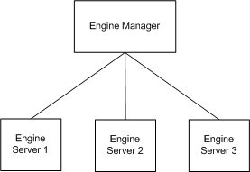
The engine server scans a portion of the forecast tree, and sends the output to the proport mechanism. The engine server masks the mdp_matrix table and processes only the nodes that are in the part of the tree relevant to its task. The ID of the task is received from the Engine Manager, which is responsible for dividing the forecast tree into smaller sub trees (called tasks).

The Engine Manager is responsible for controlling the run as a whole. Communication between the various engine modules is achieved by using the COM protocol.

Engine Components and Batch Run

The following steps describe the responsibilities of each component during a batch run of the Analytical Engine.

1. The Engine Manager creates and initializes the engine servers. Initialization includes the following steps:

   • The Engine Manager passes a callback interface to the engine servers. The engine servers will use this interface in order to make requests for new tasks to process, or to return status completion information to the Engine Manager.

   • The Engine Manager passes the database settings and all other settings to the engine servers.

   • The engine servers connect to the database and load parameters.

   • The engine servers initialize themselves using the xml schema files and request the Engine Manager for tasks to process.

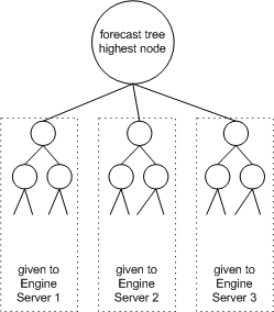
2. The Engine Manager checks if the run is a recovery run or a new run, and acts accordingly. If it is a recovery run, the Engine Manager retrieves unfinished tasks. If it is a new run, the Engine Manager resets the mdp_matrix table and allocates a forecast column. The Engine Manager divides the forecast tree into smaller tasks by updating one column in mdp_matrix that links each node with a task ID. The number of the tasks that the Engine Manager attempts to create is the number of engine servers that were initialized successfully, multiplied by a configurable factor.

3. The Engine Manager executes all the engine servers and waits for them to return a final completion status.

4. When an engine server is executing, it uses the Engine Manager callback interface in order to get task IDs to process (pull approach). The data flow between the Engine Manager and the engine servers is very low volume, containing only settings, task IDs and statuses. The data that flows between the engine servers and the database includes the sales (input) and forecasted (output) data (very high volume), forecast tree configuration information, database parameters, and certain other information.

5. The engine server uses the task ID to create a sales_data_engine table (or view) with the records for that task and then scans the forecast tree, operating select and update queries on the mdp_matrix table. During the processing of a task, an engine server filters mdp_matrix according to the task ID and operates only the subtree relating to that task. It uses two threads, one for scanning the tree and performing calculations, and one for the proport mechanism.

6. When the engine server gets a null task ID from the Engine Manager, it knows that no more task IDs are available, and it sends a completion notification to the Engine Manager.

7. When the Engine Manager has received a completion status indicator from all the engine servers, it updates the run status, executes the post process procedure, and the engine run is completed.

Details of the Distributed Engine

Your system may include the Distributed Engine, which is a mode in which the Analytical Engine automatically distributes its work across multiple machines simultaneously.

Note: For the Distributed Engine to work, the Analytical Engine must be registered on multiple machines, all of which have database client software in order to access the Demantra database.

The Distributed Engine drastically shortens the run time for a single batch engine run by processing the engine tasks in parallel, on different machines, for improved engine processing time. Also, multiple simulation requests can be handled simultaneously.

In a batch run, the Distributed Engine starts by reading a settings file that lists the machines on the network where the Analytical Engine is installed. The Engine Manager tries to instantiate an engine server on the machines in this list. Processing then continues with Step 1.