Defining Distribution Plans
This chapter covers the following topics:
- Setting Distribution Plan Options
- The Main Tabbed Region
- The Aggregation Tabbed Region
- The Organizations Tabbed Region
- The Decision Rules Tabbed Region
Setting Distribution Plan Options
This section describes how to set distribution plan options. The distribution plan options appear in the following tabbed regions:
-
Main
-
Aggregation
-
Organizations
-
Decision Rules
To access the distribution plan options:
-
If the plan name is defined: Navigate to Distribution Plans > Options
-
If the plan name is not defined: Navigate to Distribution Planner > Distribution Plans > Names. Choose your organization if prompted, define a plan name, and save your work. To access the plan options, click button Plan Options.
The Main Tabbed Region
This table describes the fields and options of the Main tabbed region:
| Object | Description |
|---|---|
| Demand Priority Rule Set | Use this option to set the Demand Priority Rule for each plan. Demand priorities are set by demand class and demand type. Priorities are assigned to sales orders and forecasts. End demand priorities are passed down the supply chain network on the dependent demands. If you prefer, you can enter priorities for each demand in the source instance or load priorities for each demand into the ODS using SQL tools. When you select the demand priority rule set in the plan options form, one of the choices is user defined priorities. If user defined priorities is selected, Distribution Planning uses the demand priorities entered for each demand. |
| Assignment Set | Use this option to select assignment set for the distribution plan. Assignment sets include the Supply Allocation rule assignment tab.
|
| Use Organization Priority Overrides | The Use Organization Priority Overrides check box is optional. However, if Use Organization Priority Overrides is checked, a demand priority rule cannot be used. Priorities are based on the organization override priorities set in the supply allocation rule for each organization-item. Allocation from a source organization to the destination organizations are based on the assigned destination organization priority.
Assign organization override priorities to the source organization to control the relative priority level of the source organization independent demands versus the dependent demands from other organizations. On demand priority override region, in supply allocation rules, you can select:
You can also include the source or shipping organization and specify a priority for the shipping organization. This allows you to specify priorities for the shipping organization when you specify priorities for the receiving organizations. If Organization Priority is selected, all unspecified warehouses are set at the same priority which is one less than any specified warehouses. For example, Organizations R1, R2 and R3 source from D2. A demand priority override is specified for R1 as 1, R2 as 2. and D2 as 2 No priority is specified for R3. The default demand priority override for R3 is 3. If no organization priority override rule is specified, then all destinations and source are treated as having the same priority. When organization priority override is used, then within an organization all demands are given the same priority. Supplies are fair shared within this priority based on the plan option customer fair share allocation method. |
| Fair Share Allocation Method: Default | For each plan, set default fair share allocation method from any source organization to the destination organizations if no supply allocation rule is specified. The three plan option choices are:
Use the default method to reduce the number of user entered fair share allocation rules. The default method is applied to all item-organizations except where a Supply Allocation Rule has been explicitly defined and assigned to the item-source organization. When the default fair share allocation method is applied to an item-destination organization, you cannot specify ranks and percents, so standard defaulting logic is used. |
| Fair Share Allocation Method: Supplier | For each plan, set the supplier fair share allocation method used for all suppliers to organizations allocation. The three plan option choices are:
Fair share allocation methods are not assigned directly to individual suppliers. The fair share allocation logic is called when supplier capacity is defined and demand exceeds available supplier capacity in an allocation bucket. Supplier capacity is fair shared to multiple organizations based on the net capacity available at the end of an allocation bucket. The total supply that is allocated is the net supply available by the end of the allocation bucket. This is based on the supplier capacity. Load consolidation for shipments from suppliers to organizations is not done. Distribution Planning uses a defaulting hierarchy for the order size multiplier for suppliers:
|
| Fair Share Allocation Method: Customer | For each plan, set customer fair share allocation method. The four plan option choices are:
Highest priority demands are allocated supplies first. When supply runs short for a particular priority, fair share allocation is performed for all demands with that priority. |
| Enable Sales Order Split | If Enable Sales Order Split is checked, and the sales order line quantity cannot be met on the suggested due date, split it into two lines as:
Sales order line splits are not preserved from one plan run to the next. Sales order line splits cannot be directly released to Oracle Order Management. You need to establish a process to update and split the sales order lines in Oracle Order Management.
|
| Enforce Supplier Capacity Constraints | If Enforce Supplier Capacity Constraints is checked, supplier capacity constraints are respected and Material Shortage exceptions are issued when supplier capacity constrains planned orders. If Enforce Supplier Capacity Constraints is not checked, supplier capacity constraints can be violated and supplier capacity overload exception messages are reported. |
| Minimum Trip Utilization % and Maximum Trip Utilization % | Use this option to set Minimum Trip Utilization % and Maximum Trip Utilization %. This option only applies to truckload ship methods. Maximum Trip Utilization: This parameter is upper limit for loading a truck. For example, if the user specifies this parameter to be 90%, then no truck is loaded over 90% of the maximum weight and cube capacities. If null, 100% is used. Minimum Trip Utilization: The planning engine generates different truckload trips with various levels of capacity utilization. Distribution plans attempt to create trips that have capacity utilization greater than the minimum truckload utilization. If null, 0 is used.
Under-utilized trip exceptions reported for trips below the minimum trip utilization %:
|
Other fields on the main tab are similar to MRP and MPS plan options. Please see the section The Main Tabbed Region for more details.
Enable Sales Order Split
In the following example, the upper table shows the sales orders before splitting and the lower table shows the Distribution Planning split of the sales orders based on supply of 100 units on Day 1 and 100 units on Day 3. Customer fair share allocation is enabled.
| Customer | Priority | Demand Quantity | Qty by Due Date | Ship Date | Due Date |
|---|---|---|---|---|---|
| Customer A | 1 | 100 | Day 1 | ||
| Customer B | 1 | 100 | Day 1 |
| Customer | Priority | Demand Quantity | Qty by Due Date | Ship Date | Due Date |
|---|---|---|---|---|---|
| Customer A | 1 | 50 | 50 | Day 1 | Day 1 |
| Customer B | 1 | 50 | 50 | Day 1 | Day 1 |
| Customer A | 1 | 50 | 0 | Day 3 | Day 1 |
| Customer B | 1 | 50 | 0 | Day 3 | Day 1 |
In this example, each sales order line is split into two lines. The Distribution Planning output shows the two lines on Day 1 have a smaller quantity and the remainder of each original sales order demand is now a new sales order line with a ship date of day 3.
These sales orders cannot be released back to Oracle Order Management. You should enable a process that allows the planner to communicate the splits to the customer service department, who can then notify the customer when the sales orders will be shipped.
The Aggregation Tabbed Region
Distribution Planning provides controls for several functional time intervals as:
-
Daily and weekly planning buckets
-
Load consolidation horizons
-
Allocation time buckets
-
Inventory rebalancing surplus days
-
Infinite time fence days
During daily planning buckets, Distribution Planning calculates supplies and demands down to the minute level. During the weekly planning buckets, Distribution Planning aggregates demands and supplies by week. Period buckets are not used in Distribution Planning.
This table describes the fields and options of the Aggregation tabbed region:
| Object | Description |
|---|---|
| Trip Consolidation Days | Trip consolidation days are days from the plan start date that trips are created, scheduled and consolidated.
|
| Trip Consolidation End Date | The Trip Consolidation End Date field is display only. It displays the end date of the trip consolidation horizon. The time stamp of the trip consolidation end date is 23:59. |
| Period Allocation Bucket | Check to enable period allocation based on the plan calendar. When checked, Daily Allocation Buckets and Weeks per Aggregate Allocation Bucket are grayed out. |
| Daily Allocation Bucket | The number of days during which the allocation bucket size is one day. Daily allocation buckets are counted against working days on the plan calendar. |
| Weekly Allocation Bucket Start Date | This field is display only and shows the start date for a weekly allocation bucket. |
| Weeks per Weekly Allocation Bucket | The number of weeks contained in each aggregate allocation bucket. |
| Inventory Rebalancing Days | The number of days that surplus inventory must be available before it can be used as supply for a demand from an inventory rebalancing relationship. Only firm supplies are considered for inventory rebalancing. Inventory rebalancing relationships are defined in the sourcing rules. Inventory rebalancing rules define a use up first relationship. Inventory is transferred from inventory rebalance sources first, thereby using up the surplus at another organization before sourcing through the usual channels. |
| Infinite Time Fence Horizon Days | Infinite time fence (infinite time fence) horizon days is the number of days from the plan start date that the supply schedule is a constraint. It is calculated based on working days in the planning calendar. If the infinite time fence start date is later than the plan horizon end date, the first day after the plan horizon end date is displayed as the infinite time fence date. After the infinite time fence start date, the distribution planning engine behaves as follows:
|
| Infinite Time Fence Start Date | The first date of the Infinite Time Fence. |
Please see the section Inventory Rebalancing for more details.
Daily Allocation Buckets
Daily allocation buckets are the number of buckets during which the allocation bucket size is one day.
Null or zero value means that there are no daily allocation buckets. For example, if the plan start date is on a Wednesday and week ending date is Sunday, the first weekly allocation bucket is short two days.
You must specify that the number of daily allocation buckets is less than or equal to the number of daily planning buckets.
Weeks per aggregate allocation bucket is the number of weeks contained in each aggregate allocation bucket. It can be an integer only. If the weeks per aggregate allocation bucket is two or more, then the last allocation bucket may not contain that number of weeks (depending on how many weeks are left before the plan horizon end date). For example, if weeks per allocation bucket is two, but the plan horizon only allows one week in the last allocation bucket, only one week is used.
The plan horizon is not extended because of the allocation buckets. If there are daily allocation buckets, the aggregate buckets start on the next week start date and additional daily allocation buckets may be used. For example, if the daily allocation buckets end on a Thursday and the week start date is Monday, one additional daily allocation bucket is used (assuming that Saturday and Sunday are non-working days).
Supply allocation proceeds bucket by bucket. Demands in the first bucket (daily, weekly or period) are sorted by priority and firm demands are given the highest priority. Within the bucket, for each demand of a priority:
-
Demands are allocated supplies on or before the demand date
-
Or if not available by the demand date, then by the bucket end date
-
Or if a shortage occurs for a demand priority within an allocation bucket, the supplies are fair shared based on the supply allocation rules and plan options
Unsatisfied demands are carried forward to the next allocation bucket
Trip Consolidation Days
Trip consolidation days sets the trip scheduling horizon. Trips consist of internal sales orders and internal transfers that are scheduled with the same ship date, dock date, and ship method.
Distribution Planning selects ship methods by working through the list of available ship methods. The list is sorted by rank (lowest value first), cost (lowest cost first using the costs specified on the inter-organization ship methods form), in transit time (shortest in transit time first), and then maximum trip weight (highest value first).
After a ship method is selected for the first internal transfer, calculate the earliest the trip can ship based on the supply availability and the latest the trip could possibly arrive based on the destination inventory requirements. Continue loading the trip with additional supplies that fit within the trip earliest possible ship date and latest possible dock date.
Distribution Planning uses the following rules when consolidating trips:
-
Safety stock level: distribution planning will always ship available supplies on time to meet safety stock demands. Minimum Trip Capacity can be violated.
-
Target level: During trip consolidation, distribution planning will only ship available supplies on time to meet target inventory levels if there is a trip that the supply can be put on without violating the trip capacity.
-
For a supply, the earliest possible ship date considers the destination maximum inventory level constraint.
-
For a supply, the latest possible dock date considers the source maximum inventory level constraint.
Trip Identifiers
Trips are identified in the trips form and the supply and demand window with trip numbers. Trip identifiers appear in the Distribution Planning Trips form and the supply and demand window. Internal sales orders and internal requisitions on a trip have the same ship and dock date and ship method. Transfers are grouped based on the load consolidation limits for a ship method Trips are created within the load consolidation horizon.
Trip identifiers are not released to the source instance, only the internal sales orders and internal requisitions which make up the trip are released to the source instance.
If an internal transfer is too big for the maximum trip size, then the internal transfer is automatically split into two or more internal transfers where each internal transfer is now the maximum trip size or lower. Automatic splitting of internal transfers into smaller sizes to meet the maximum trip size constraint occurs in one of two cases:
-
If the selected ship method maximum trip size would be violated, then the internal transfer can be split into multiple internal transfers so that the trips are below the maximum trip size. For example, if the internal transfer is for 1000 units and 200 units fill a semi-trailer, then 5 internal transfers are created.
-
For ship methods that do not have a maximum trip size, internal transfers are not split.
The Trips Form
The Trips form displays details about each trip including the from and to organizations and the ship and dock dates and the ship method. The weight and cube utilization are calculated and displayed in percents if trip limits are defined for the ship method.
Other fields shown include trip weight and cube, available weight and cube, and maximum weight and cube. Also included for each trip are the in transit lead-time, the ship method, mode, service level and carrier name. Statuses for each trip are provided to show if it is an existing trip and if there are trip utilization exceptions issued for it.
The following is calculated for each trip and displayed in the trips form:
-
Earliest supply date: The earliest possible date that a trip can ship based on the material available dates of all of the supplies on the trip. Tells the planner that a trip can ship earlier than scheduled. For demands, the material available date means when the supplies pegged to the demand are complete and available for shipping.
-
Latest possible dock date: The latest of all of the required dock dates for the supplies scheduled on the trip. Tells the planner when the trip should arrive at the destination organization. If it is earlier than the actual scheduled dock date, it indicates that the trip requires expediting.
-
Cost of under utilization: The formula is Trip Upper Weight Limit * (cost/weight unit) - Actual Trip Weight * (cost/weight unit). Applies when the cost/unit for weight is provided on the inter-organization shipping form.
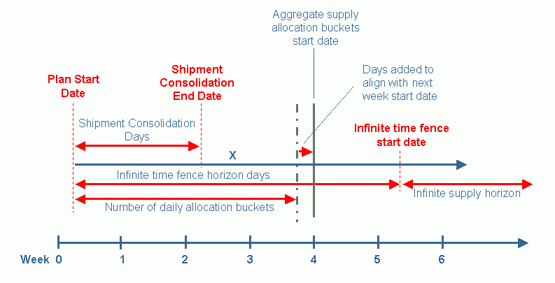
Understanding Time Aggregation Options
This diagram illustrates the relationship among the trip consolidation time fence, the trip consolidation days, the infinite time fence, and the daily/aggregate allocation buckets. In this example, the planning buckets are daily.
The Organizations Tabbed Region
You can specify a distribution plan as a supply schedule to other distribution plans. This enables you to subset the distribution planning problem and run multiple distribution plans. You can run a centralized allocation plan less frequently and run replenishment plans for the outlying locations more frequently. The behavior of a distribution plan as a supply schedule is exactly the same as the behavior of MPP/MPS/MRP plans as supply schedules.
For items and organizations planned in the central plan, no new supplies are planned when it is used as a supply schedule. Instead, the available supplies are pushed further outwards in the supply chain and may be reallocated during subsequent runs of the distribution plan. The only difference is after the infinite time fence.
Distribution plans can be fed as a demand schedule to a distribution plan. This allows distribution planning users to also subset the planning problem into multiple distribution plans, and close the loop between plans by feeding the main distribution plan as a demand schedule. When a distribution plan is listed as a demand schedule for an organization in a second distribution plan, the behavior is similar to checking the interplant check box on an Oracle Advanced Supply Chain Planning plan. The only demands passed are the requested outbound shipments for the organization. The demands from the demand schedule plan appear in the distribution plan as inter-organization demand.
Setting Up the Organizations Tabbed Region
-
Enter global demand schedules from Demand Planning.
-
Check or uncheck the Include Sales Order check box.
WIP, Reservations, and Purchases are always included. Safety stocks are always planned.
-
Add demand and supply schedules.
Distribution plans can be used as demand schedules. Distribution plans and MRP/MPS/MPP plans can be supply schedules.
Distribution plans do not create any new planned orders for item-organizations that are found in an MRP/MPS/MPP supply schedule or a Distribution Plan supply schedule until the infinite time fence. If there are existing non-firm supplies for that item-organization that are not in the supply schedule, these are canceled by default since the distribution plan relies on the supply schedule. If the existing supplies are firm, then the distribution plan does not cancel them.
The Decision Rules Tabbed Region
When the MSO: Enable Decision Rules is set to Yes, you can select Decision Rules options for Distribution Planning in the Decision Rules Tab. This tab is grayed out if you have set MSO: Enable Decision Rules to No.
Decision rules are supported by Distribution Planning for:
-
End item substitution
-
Substitute components
-
Alternate BOMs
-
Alternate sources