1 Overview to Forecasting
This chapter contains these topics:
Effective management of distribution and manufacturing activities begins with understanding and anticipating the needs of the market. Implementing a forecasting system allows you to quickly assess current market trends and sales so that you can make informed decisions about your company.
Forecasting is the process of projecting past sales demand into the future. An accurate forecast helps you make operations decisions. For this reason, forecasting should be a central activity in your operations. You can use forecasts to make planning decisions about:
-
Customer orders
-
Inventory
-
Delivery of goods
-
Work load
-
Capacity requirements
-
· Warehouse space
-
· Labor
-
· Equipment
-
-
Budgets
-
Development of new products
-
Workforce requirements
The Forecasting system can generate the following types of forecasts:
-
Detail forecasts - Detail forecasts are based on individual items.
-
Summary forecasts - Summary (or aggregated) forecasts are based on larger groups, such as a product line.
-
Planning bill forecasts - Planning bill forecasts are based on groups of items in a bill of material format that reflect how an item is sold, not how it is built.
1.1 System Integration
Forecasting is one of many systems that make up the Enterprise Requirements Planning and Execution (ERPx) system. Use the ERPx system to coordinate your inventory, raw material, and labor resources to deliver products according to a managed schedule. ERPx is fully integrated and ensures that information is current and accurate across your business operations. It is a closed-loop manufacturing system that formalizes the activities of company and operations planning, as well as the execution of those plans.
The following systems make up the JD Edwards World ERPx product group.
Figure 1-1 Systems in the JD Edwards ERPxE Product Group
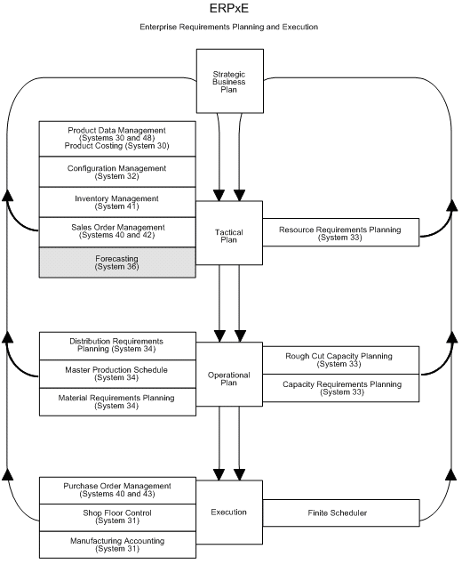
Description of "Figure 1-1 Systems in the JD Edwards ERPxE Product Group"
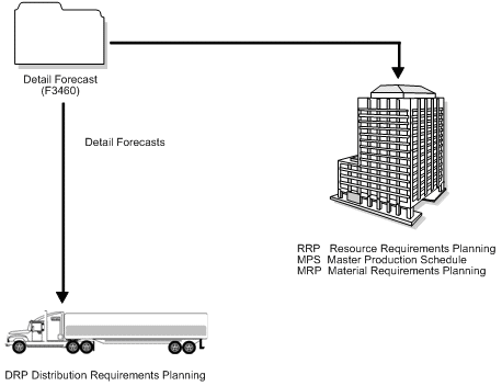
The Forecasting system generates demand projections that you use as input for JD Edwards World planning and scheduling systems. These systems calculate material requirements for all component levels, from raw materials to complex subassemblies.
The Resource Requirements Planning (RRP) system uses a forecast of future demand to estimate the time and resources needed to make a product.
The Master Production Schedule (MPS) system plans and schedules what a company expects to manufacture. Data from the Forecasting system is one MPS input that helps determine demand before you execute production plans.
Material Requirements Planning (MRP) is an ordering and scheduling system that explodes the requirements of all MPS parent items to the components. You can also use forecast data as demand input for lower-level MRP components that are service parts with independent demand (demand not directly or exclusively tied to production of a particular product at a particular branch or plant).
Distribution Requirements Planning (DRP) is a management system that plans and controls the distribution of finished goods. You can use forecasting data as input for DRP so you can more accurately plan the demand that you supply through distribution.
1.2 Features
You can use the Forecasting system to:
-
Generate forecasts
-
Enter forecasts manually
-
Maintain both manually entered forecasts and forecasts generated by the system
-
Summarize the sales order history data in weekly or monthly time periods
-
Generate forecasts based on any or all of 12 different formulas that address a variety of forecast situations you might encounter
-
Calculate which of the 12 formulas provides the best fit forecast
-
Define the hierarchy that the system uses to summarize sales order histories and detail forecasts
-
Create multiple hierarchies of address book category codes and item category codes, which you can use to sort and view records in the detail forecast table
-
Review and adjust both forecasts and sales order actuals at any level of the hierarchy
-
Integrate the detail forecast records into DRP, MPS, and MRP generations
-
Force changes made at any component level to both higher levels and lower levels
-
Set a bypass flag to prevent changes generated by the force program being made to a level
-
Store and display both original and adjusted quantities and amounts
-
Attach descriptive text to a forecast at the detail and summary levels
-
Forecast up to five years, based on the processing options settings
-
Import or export data
Flexibility is a key feature of the JD Edwards World Forecasting system. The most accurate forecasts take into account quantitative information, such as sales trends and past sales order history, as well as qualitative information, such as changes in trade laws, competition, and government. The system processes quantitative information and allows you to adjust it with qualitative information. When you aggregate, or summarize, forecasts, the system uses changes that you make at any level of the forecast to automatically update all other levels.
You can perform simulations based on the initial forecast, which allows you to compare different situations. After you accept a forecast, the system updates your manufacturing and distribution plan with any changes you have made.
1.2.1 Forecasting Levels and Methods
You can generate both single-item (detail) forecasts and product line (summary) forecasts that reflect product demand patterns. Select from 12 forecasting methods, and the system analyzes past sales to calculate the forecast. The forecast includes detail information at the item level and higher-level information about a branch or the company as a whole.
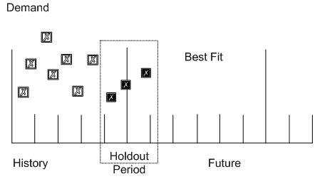
The system recommends the best fit forecast by applying the selected forecasting methods to past sales order history and comparing the forecast simulation to the actual history. When you generate a forecast, the system compares actual sales order histories to forecasts for the months or weeks you indicate in the processing option and computes how accurately each of the selected forecasting methods would have predicted sales. Then, the system recommends the most accurate forecast as the best fit.
The system determines the best fit in the following sequence:
-
The system uses each of the methods that you selected in processing options to simulate a forecast for the holdout period. Refer to Appendix A - Forecast Calculation Examples, for a definition of holdout period.
-
The system compares actual sales to the simulated forecasts for the holdout period.
-
The system calculates the percent of accuracy or the mean absolute deviation to determine which forecasting method closest matched the past actual sales. The system uses the percent of accuracy or the mean absolute deviation based on the processing options that you select.
-
The system recommends a best fit forecast by the percent of accuracy that is closest to 100% (over or under) or the mean absolute deviation closest to zero.
The Forecasting system uses 12 methods for quantitative forecasting. The system also indicates which of the methods provides the best fit for your forecasting situation.
1.2.2 Demand Patterns
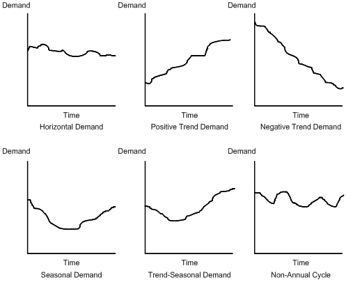
The Forecasting system uses sales order history to predict future demand. Different examples of demand follow. Forecast methods available in the JD Edwards World Forecasting system are tailored for these demand patterns.
You can forecast the independent demand of the following items for which you have past data:
-
Samples
-
Promotional items
-
Customer orders
-
Service parts
-
Inter-plant demands
You can also forecast demand for the following item types determined by the manufacturing environments in which they are produced:
-
Make-to-stock - End items to meet customers' demand that occurs after the product is completed
-
Assemble-to-order - Subassemblies to meet customers' option selections
-
Make-to-order - Raw materials and components stocked in order to reduce lead time
1.2.3 Forecast Accuracy
The following statistical laws govern the accuracy of a forecast:
-
A short-term forecast is more accurate than a long-term forecast, because the farther into the future you project the forecast, the more variables can impact the forecast.
-
A forecast for a product family tends to be more accurate than a forecast for individual members of the product family. Some errors cancel as the forecasts for individual items summarize into the group.
1.3 Forecast Considerations
You should not rely exclusively on past data to forecast future demands. The following circumstances might affect your business and require you to review and modify your forecast:
-
New products that have no past data
-
Plans for future sales promotion
-
Changes in national and international politics
-
New laws and government regulations
-
Weather changes and natural disasters
-
Innovations from competition
-
Economic changes
You might use any of the following kinds of long-term trend analysis to influence the design of your forecasts:
-
Market surveys
-
Leading economic indicators
-
Delphi panels
1.4 Forecasting Process
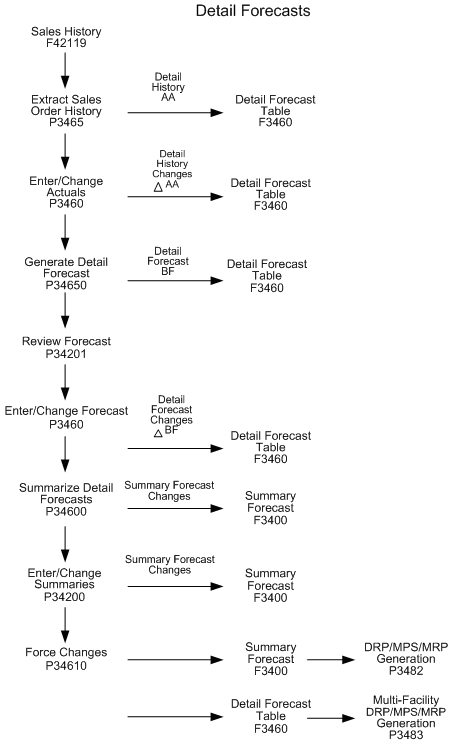
You use Extract Sales Order History to copy data from the Sales History table (F42119) into either the Detail Forecast table (F3460) or possibly the Summary Forecast (F3400) table, depending on the kind of forecast you plan to generate.
You can generate detail forecasts or summaries of detail forecasts based on data in the Detail Forecast table. Data from your forecasts can then be revised. The process is illustrated in the following graphic.
The following graphic illustrates the sequences you follow when you use the detail forecasting programs.
