Creating a Demand Variability Process
This chapter describes the creation of a demand variability process.
This chapter covers the following topics:
Creating a Demand Variability Process
Overview
A demand variability process is a database procedure (named COMPUTE_STD_ERR) that calculates the demand variability (or standard error) between two specified series, at specified aggregation levels. You run this procedure from a Workflow using the Stored Procedure Step that runs COMPUTE_STD_ERR. Use the demand variability process as an input to a safety stock calculation, or to determine what safety stock levels are needed to meet demand according to a predefined service level and replenishment cycle.
Aggregation Levels Used in Demand Variability Calculation
When you calculate demand variability, you specify two aggregation levels. The demand variability is calculated for each combination of those two levels. You can use the following combinations of levels:
-
Item level and location level
-
Item level and matrix level
-
Location level and matrix level
-
Matrix level and another matrix level
The target series (which you define to display the result of the calculation) must be defined on the corresponding dimension in the mdp_matrix table.
To create a demand variability profile
-
Start the Business Modeler.
-
From the Configuration menu, choose Configure Demand Variability Calculation.
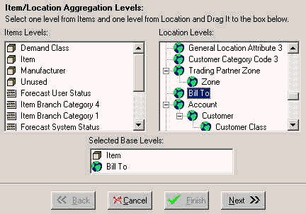
The wizard displays a screen where you specify the aggregation levels where the demand variability is to be calculated.

This screen displays two lists of aggregation levels. The left list contains all the item levels and all the matrix levels. The right list contains all the location levels and all the matrix levels.
-
Specify the levels as follows:
-
Drag a level from each list to the Selected Base Levels field at the bottom of the screen.
-
To remove a level from the Selected Base Levels field, right-click and then select Delete the Level.
-
-
Click Next.
The wizard displays a screen where you specify the range of dates for which the demand variability is to be calculated.

-
Specify dates as follows:
-
In the From Date spin box, select the number of base time buckets by which to go back. This is the date from which demand variability is to be calculated.
-
In the To Date spin box, select the number of base time buckets by which to go back. This is the date to which demand variability is to be calculated.
-
-
Click Next.
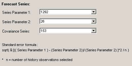
The wizard displays a screen where you specify the series to use in the calculation.

-
Specify the forecast series as follows:
-
In Series Parameter 1, select the series to use as Series Parameter 1 in the standard error formula.
-
In Series Parameter 2, select the series to use as Series Parameter 2 in the standard error formula.
-
In Covariance Series, select the mdp_matrix series to use as the standard error calculated for the combination.
-
-
Click Next.
The wizard displays a screen where you can review your choices.
-
Do one of the following:
-
To change a setting, click Back repeatedly until you reach the screen that has the setting. Then change it as needed.
-
When you are finished, click Finish. The wizard then creates a database procedure named COMPUTE_STD_ERR. You must run this procedure from a Workflow (use the Stored Procedure Workflow step).
-
To cancel without saving changes, click Cancel.
-
Generating Safety Stock
Once calculated, the demand variability can be used to drive a simple safety stock calculation in Demantra. A series can combine the demand variability with a desired service level and the replenishment time associated with the time and generate a suggested safety stock. An example for such a series in a weekly system would have the expression:
-
consensus plan * z_val ( service level) * demand variability * sqrt ( ( repl cycle / 7 ) )
where consensus plan, service level, demand variability and, replenishment cycle are all series.
If the requirement calls for a more complicated safety stock calculation, Oracle Inventory Optimization can be used.