Understanding Activity-Based Management Models, Modeling Components, and Rate Types

This chapter discusses:

• Activity-Based Management modeling components.

• Using Activity-Based Management models.

• Using rates with your Activity-Based Management model.

• Creating interunit models for shared services.

• Modeling for manufacturing purposes.

• Modeling for service-related industries.

• Modeling with Activity-Based Planning and Simulation (ABPS).

Activity-Based Management Modeling Components

Activity-Based Management uses models—complete sets of rules to define individual activity-based costing model objects and their relationship to your organization's financial management system, primarily the general ledger. Models let you specify different business scenarios for comparative analysis. Activity-Based Management lets you define, run, and analyze models to assess your organization's profitability.

Create models in Activity-Based Management by defining the following components:

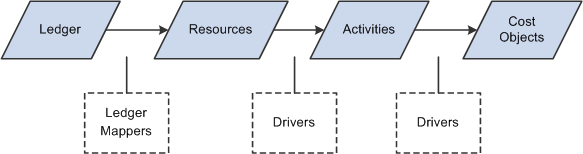
Modeling components

Resources

Resources—such as people, facilities, and costs associated with people and expenses—are the economic elements consumed while performing activities. They are the core elements that let your organization operate.

Activities

Activities consume resources and drive costs to cost objects. The lowest-level definition of what your organization does, activities are the foundation for measuring activity costs.

Cost Objects

Cost objects represent cost information grouped by profitability dimensions—products, customers, and channels. With your model's resources and activities linked to cost objects, which are the final results of the activities performed by your organization, they are often the focal point of profitability analysis.

Ledger Mappers

Ledger mappers relate expense data from your general ledger accounts to resource objects. You can map multiple ledger line item amounts to one or more resource IDs in the following two ways:

• An actual amount that represents actual costs of the accounting period results

• A budgeted amount that you can use to calculate the capacity rates as well as budgeted model results

Drivers

Drivers—transactional, duration, and intensity—let you assign monetary amounts from one object to another throughout the model (calculated by amount, percentage, spread even, and direct) in different ways depending on assignment type and object type. You can even assign drivers across business units.

Pointers

Pointers specify the location of driver quantities in the Operational Warehouse - Enriched (OWE) tables. Rather than entering and maintaining static driver quantities, pointers let you to extract values from any location in the OWE, and then use these values as driver quantities.

Using Activity-Based Management Models

The foundation of Activity-Based Management is the ability to create models that replicate your organization's business processes so that you can analyze how costs flow through your customers, departments, and channels, thus letting you increase your understanding of the relationships between resources, activities, and cost objects.

To use a model in Activity-Based Management, first define it within the system by selecting a rate type that specifies how Activity-Based Management should calculate the monetary amounts for each object in the model.

Using Rates with Your Activity-Based Management Model

While most activity-based costing systems calculate resource, activity, and cost object results using actual or budgeted historical data, Activity-Based Management offers capacity and frozen rates as well. This section discusses the following rate options for model types:

• Actual

• Budgeted

• Capacity

• Frozen

• Combination

These rate options let you create and run basic, full-absorption models that have the following advantages:

• They calculate variances from actual costs such as spending, volume, and capacity variances.

• They attribute monetary amounts to entities that operate at greater than or less than their capacity.

• They maintain a more constant consumption pattern over multiple time periods.

Actual Rates

Ledger mappers move actual amounts mapped from the general ledger into resource objects of the Activity-Based Management engine, which tracks data related to actual driver quantities:

Calculating actual rates

The actual rate type assumes that operations are occurring at 100 percent capacity.

A rate represents a monetary amount divided by a driver quantity. To calculate an actual rate, Activity-Based Management applies the following formula to the values captured by the model:

(Actual Rate) = (Actual Monetary Amount) / (Actual Driver Quantity)

Note. This rate type can fluctuate temporarily with general ledger fluctuations and does not address capacity.

Budgeted Rates

Ledger mappers move budgeted amounts mapped from the general ledger into resource objects of the Activity-Based Management engine, which tracks data related to budgeted driver quantities:

Calculating budgeted rates

Because a rate represents a monetary amount divided by a driver quantity, Activity-Based Management calculates the budgeted rate by applying the following formula to arbitrary values captured by a model:

budgeted rate = budgeted amount / budgeted driver quantity

Determining both the actual and budgeted rates let you calculate two variance types:

As a result, you can calculate the following two types of variance results:

The combined results create the total variance. If you apply the budgeted rate calculated by the Activity-Based Management engine, only those values pass through the remainder of the model versus passing along the actual amount.

The following diagram illustrates how the system calculates volume and spending variance:

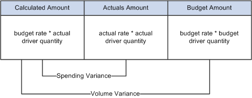
Variance calculation for actual and budgeted rates

Note. As with the actual rate, the budgeted rate also does not address capacity and is subject to fluctuations based on general ledger fluctuations.

Capacity Rates

Actual and budgeted driver quantities can and do fluctuate over time; likewise, the actual and budgeted rates fluctuate over the same time period. Because decisions made on the basis of these fluctuating rates could be misleading, the concept of capacity rates becomes important.

When entities are not operating at their full capacity and all costs are applied to activities and cost objects, the model fully absorbs the costs and managers are forced to use historical information to make decisions.

Activity-Based Management lets you assign the excess costs to a departmental cost object so that you can track excess capacity. Assigning excess capacity to such an object balances the actual amounts within the model, and the flow of amounts through the objects remains constant:

Calculating capacity rates

The capacity rate is the result of the budgeted amount divided by the capacity driver quantity:

capacity rate = (budgeted monetary amount) / (capacity driver quantity)

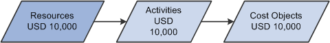
Example of a Capacity Calculation

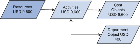
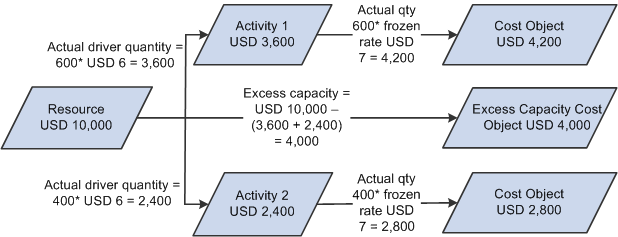
Suppose that the actual resource cost mapped from the general ledger is 10,000 USD. Our actual driver quantity for activity 1 is 600 units; for activity 2 it is 400 units. In addition, suppose that the budgeted amount for the resource is 9,600 USD, and the capacity volume for the resource is 1,600.

The system calculates a capacity rate by dividing the budget amount value by the capacity volume quantity as follows:

9,600 USD / 1,600 = 6.00 USD

Values going to activity 1 and activity 2 are then calculated by multiplying the actual driver quantities by the capacity amount.

Activity 1 actual driver quantity = 600 x 6 USD = 3,600

Activity 2 actual driver quantity = 400 x 6 USD = 2,400

For the model to balance, the system places the excess amount in the departmental excess capacity cost object. The resource total is 10,000 USD while activities total 6,000 USD. The system places the remaining 4,000 USD in the excess capacity cost object:

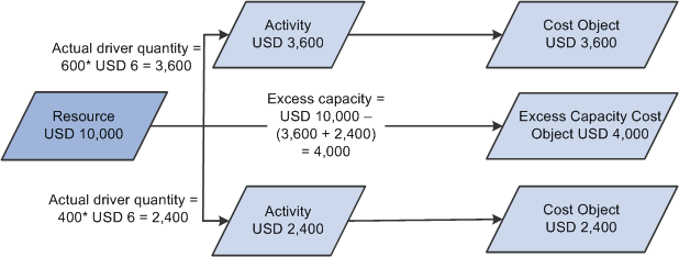
Capacity rate calculation example

When defining the model, it is important to determine where in the data flow the capacity calculation will occur. You can calculate capacity at either the resource or activity driver level in a single data flow. It cannot exist in both the resource driver and activity driver levels of a single data flow. A model can consist of several data flows.

The following diagram illustrates a single model containing two data flows where data flow 1 could have the calculation occur at the resource driver level and data flow 2 could have the calculation occur at the activity driver level:

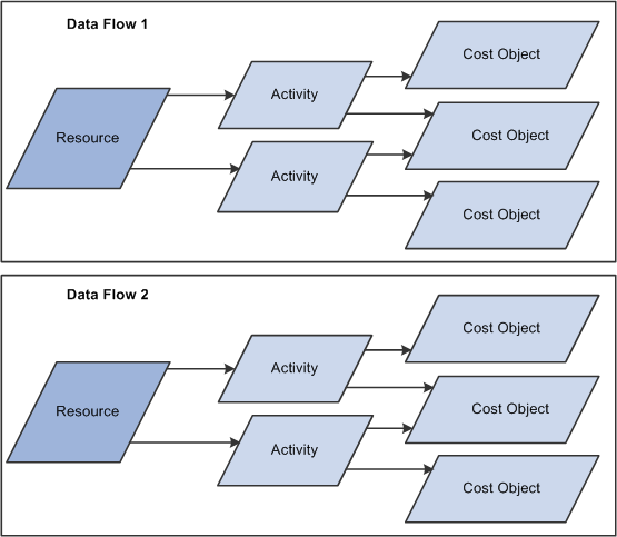
Example of an Activity-Based Management model with two data flows

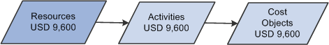
Frozen Rates

A frozen rate is fixed and agreed upon outside the context of the Activity-Based Management model:

Calculating frozen rates

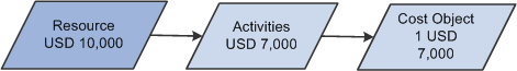
Example of a Frozen Rate Calculation

Using a frozen rate lets you calculate variances from actual, budgeted, or capacity values. Because information about the driver quantity is not used to calculate the rate, the variance is not divided between spending and volume:

Frozen rate calculation example

The following diagram shows the variance calculation using a frozen rate:

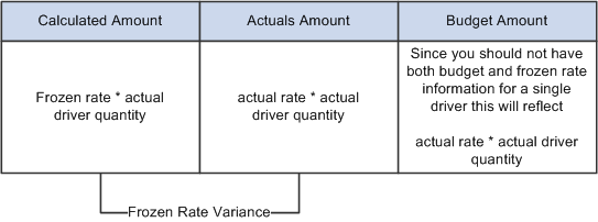
Frozen rate variance calculation

Combination Rates

Combination rates let you combine a mixture of actual, budgeted, capacity, and frozen rate information. Here's an example of the calculation of data flow for a combination model:

Calculation data flow example for a combination model type

Creating Interunit Models for Shared Services

What happens if you need several models for shared services? For example, suppose that your business unit has two production sites and a central administrative office supporting the two production sites. In traditional activity-based costing, the only way to model this is by making a single, large model for the entire business unit. This makes the scope of the project large and complicated. However, with Activity-Based Management, you can use an interunit, shared-service model to address this business requirement.

Activity-Based Management lets you cost services provided by a shared-services business unit or a shared-services group into a separate model. After you determine these shared-services cost objects, assign those costs to other models within or outside the same business unit.

Perhaps one of the shared services, provided by the example's central administrative office, is the human resources function. Because you need to drive human resources amounts between models, while you're creating a model you make Hiring Personnel a cost object. After you finish building your model, run the model and derive a total monthly cost for the Hiring Personnel cost object.

Suppose that, for example, Site A is an older facility and does not require many new hires; in fact, Site A hired only two people last month. Site B, however, is a rapidly growing facility and hired 18 people last month. This disparity could lead you to define an interunit driver that assigns 10 percent of the cost of hiring to Site A and 90 percent to Site B. This type of driver lets you make assignments from the cost object of one business unit and model to the support activities of one or more business units and models.

You can allocate shared-service resource costs to other shared-service resources using the looping method, which can produce more accurate results because the system bases the allocation on the processes that the resource performs. Once the allocation is complete, the cost from the cost object loops to the corresponding resource and continues looping until the percentage difference between the cost resource and the corresponding cost object meets a tolerance limit or exceeds a maximum loop amount. Once reciprocal allocations are complete, the system sends final costs to a production Activity-Based Management model using the existing inter-business unit (IBU) drivers.

Understanding Reciprocal Allocation and Looping

Reciprocal allocation in Activity-Based Management models lets you allocate shared-service resource costs to other shared resources. Define a single, shared-service model that includes all reciprocal Activity-Based Management objects and activities. Once reciprocal allocations are complete, the system sends final costs to a production Activity-Based Management model using the existing IBU drivers.

Within the shared-service model, define a cost object with the same name as the resource. The system bases the allocation on the processes that the resource performs. Once the allocation is complete, the cost from the cost object loops to the corresponding resource and continues looping until the percentage difference between the cost resource and the corresponding cost object meets a tolerance limit or exceeds a maximum loop amount. You can allocate any residual cost remaining after looping is complete because the targets of residual amounts often serve as sources for further allocations.

Understanding Reciprocal Allocation Methods

Activity based costing drives overhead costs from resources to activities and then to the cost objects. Activity based costing can also drive costs directly from resources to cost objects. In scenarios where costs require allocations among resources (reciprocal allocations), activity based costing drives costs to activities only after completing allocations to the resources. For example, IT and HR resources could share costs with each other. Therefore, the actual cost of these resources can be determined only after they complete the allocation of costs to each other.

The following example shares costs between resource 'S' and resource 'T.' In addition, it allocates the resource cost of 'S' to cost objects 'U,' 'V,' and resource 'T' (40%, 40% and 20% respectively) and drives resource cost of 'T' to objects 'V,' 'W,' and resource 'S' (20%, 50% and 30% respectively).

There are two methods of performing a reciprocal allocation:

• Mathematical (simultaneous equation)

• Iterative

These methods are discussed below.

Mathematical Method

The following algebraic equation models our example for simplistic reciprocal allocations:

• S = 100 + .3T

• T = 200 + .2S

Solving for S and T gives S = $170.21 and T = $234.04.

The following steps demonstrate a reciprocal allocation:

Allocate the cost of resource S to objects U, V and resource T (40%, 40% & 20% respectively).

Allocate the cost of resource T to objects V, W and resource S (20%, 50% & 30% respectively).

Iterative Method

With the iterative method, you repeat allocations until the resource amounts for S and T become negligible or zero. This method is most suited for computer applications. When the resource amounts become negligible (as defined by a tolerance limit attribute), the program exits the iterative allocation loop.

The following steps demonstrate an iterative allocation:

Allocate the cost of resource S to objects U, V and resource T (40%, 40% & 20%, respectively).

Allocate the cost of resource T to objects V, W and resource S (20%, 50% & 30%, respectively).

Iteration 1 starts by allocating resource costs of S ($100) and T ($200). After allocation, resources S and T have reciprocal allocation amounts of $60 and $20 respectively.

After Iteration 2, resources S and T have reciprocal amounts of $6 and $12, respectively.

We repeat the allocations until the allocating resource amounts are near zero (which occurs in Iteration 8).

Modeling for Manufacturing Purposes

Activity-Based Management lets you use routing information from manufacturing to set up activity driver information within the system. Activity-Based Management can determine which activity is performed on which cost objects along with the quantifiable measures for that relationship. It uses Bill of Materials (BOM) information from manufacturing and transforms the components within the BOM hierarchy into cost objects in Activity-Based Management. In addition, Activity-Based Management can maintain the BOM structure. This is important because, once the Activity-Based Management calculation is finished, each component contains cost information. The roll-up of these costs using BOM hierarchy results in a total indirect cost of the resources, activities, and cost objects. Then, the indirect cost information calculated from Activity-Based Management output is directed back to the PeopleSoft Cost Management environment.

To set up models for manufacturing purposes, create a combination model and start the Routing Information engine to set up your drivers.

Modeling for Service-Related Industries

Service industries typically offer a wide range of products. Banks, for example, have many types of checking and savings accounts, home mortgages, and car loans. Cable television companies tend to offer many packages such as basic and standard services, premium packages with selections of movie channels, and digital cable channel packages. Each product or service has its own unique characteristics requiring different demands on the providing organization's resources. Essentially, all of the operating costs associated with the products from any service organization are determined by its customers' behavior.

To determine costs for services, Activity-Based Management lets you model for Bill of Services (BOS). BOS is a collection of product and service costs for customers. This collection of costs, which can be a unique combination of standard products and services, lets you create new service packages and, in turn, new business opportunities to serve your customers.

BOS functionality includes the ability to create new and unique combinations of standard services and combine them into a package service. It also includes functionality to apply a standard rate to the new services provided to estimate new business opportunities and costs to serve a customer. Based on data from pre-existing or new package services, you can manipulate the volume, adjust to the correct customer demand for those services, and eventually calculate the resource requirements for the new changes in demand.

Modeling with ABPS

The ABPS feature of Activity-Based Management lets you forecast values for your models. Using ABPS functionality, you can make decisions on resource requirements based on factual data for product demand, resource efficiency, activity efficiency, and activity rate cost.

See Also

Understanding ABPS