Lesson: Pivoting Rows and Columns

  To pivot Year data from a row group to a column group:

1. Select File, and then New or click .

2. Select Essbase, and then Retrieve.

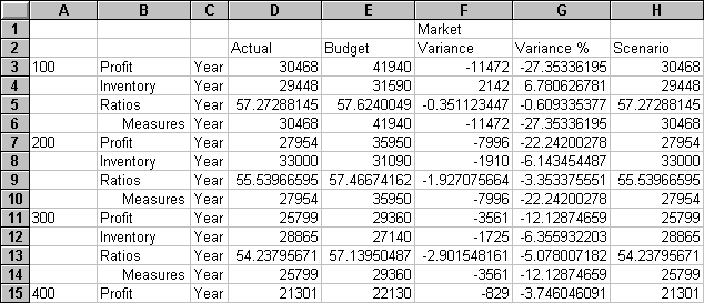
3. Drill down (double-click) on Measures and Product (in cells B1 and C1, respectively).

4. Press Alt, and, in cell E1, drill down (double-click) on Scenario.

   

5. In cell C3, select Year.

6. Select Essbase, and then Pivot.

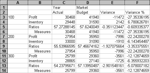
   Essbase pivots the Year dimension to a column group next to Market (above the Scenario members).

   

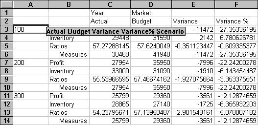
7. As another example, in cell C2, select Actual.

8. Right click and drag Actual to product 100 in cell A3.

   

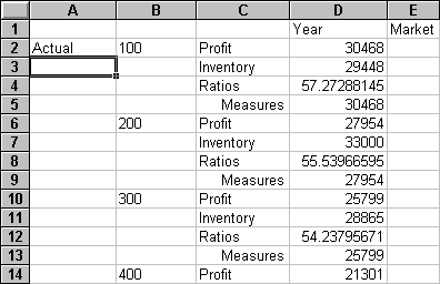
   When you pivot the Scenario members (Actual, Budget, Variance, and Variance%) from a column group to a row group, the row group is displayed to the left of the Product members:

   

  To transpose the order of row groups:

1. In cell A2, select Actual.

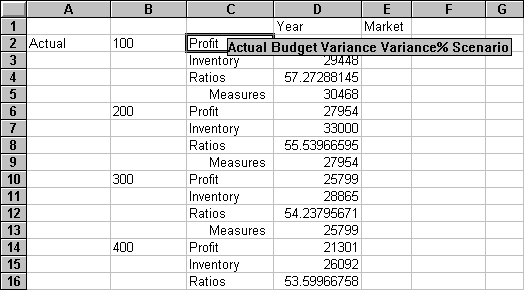
2. Right-click and drag Actual to Profit in cell C2.

   The spreadsheet before the pivot operation:

   

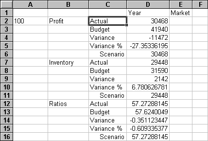
   The pivot changes the order of the row groups:

   

   In this example, notice that the source cell and the destination cell are now members.