Highlighting Pivot Table metric values that fall within a specified range

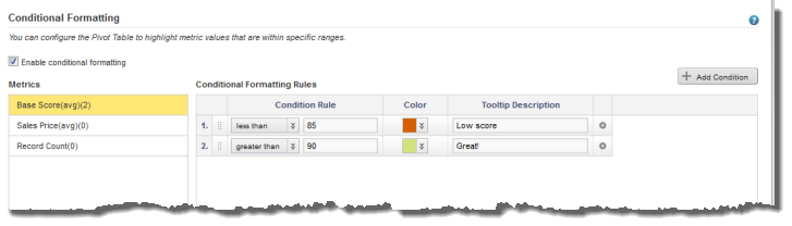
The Conditional Formatting tab of the Pivot Table edit view allows you to highlight specific metric values.

To configure whether to use conditional formatting, and select the values to highlight:

1. To allow conditional formatting, make sure that the Enable conditional formatting checkbox is checked. It is checked by default.

   If the checkbox is not checked, then there is no conditional formatting.

2. In the Metrics list, click the metric for which to configure conditional formatting.

   For each metric, the list displays the number of conditional formatting rules created for it.

3. To add a new range of values to highlight for that metric, click Add Condition.
4. To configure a condition:
   1. From the Condition Rule type drop-down list, select the type of comparison.
   2. In the field (or fields, for the "is between" option), enter the value(s) against which to do the comparison.

      Note that for the "is between" option, the values are inclusive. So if you specify a range between 20 and 30, values of 20 and 30 also are highlighted.

   3. From the Color drop-down list, select the color to use for the highlighting.
   4. In the Tooltip Description field, type the text to display in the tooltip for a highlighted cell.
5. The conditions are applied based in the order they are listed. So a condition at the top of the list has a higher priority than a condition lower in the list.

   To change the priority of the conditions, drag and drop them to the appropriate location in the list.

6. To remove a condition, click its delete icon.