Setting Up Curve Sets

This section provides an overview of operation codes and discusses how to:

Define the curve sets data sources.
Define the curve sets market issues.
Define the curve sets derived data.
Define the curve sets generic data.

To set up curve sets, set up the Data Source page. On this page, you specify the data type that you use. This data type field determines which of the following additional pages you set up:

Generic Data page.
Market Issues page.
Derived Data page.

Pages Used to Set Up Curve Sets

Page Name	Definition Name	Navigation	Usage
Data Source	YC_DATA_SRC_PNL	select Financial Services Industries, then select Interest Rate Environment, then select Dataset Definition, then select Curve Sets, then select Data Source	Set up the data source within the system.
Generic Data	YC_GENERIC_PNL	select Financial Services Industries, then select Interest Rate Environment, then select Dataset Definition, then select Curve Sets, then select Generic Data	Use when creating term structures from generic data sets.
Market Issues	YC_MRKTYIELD_PNL	select Financial Services Industries, then select Interest Rate Environment, then select Dataset Definition, then select Curve Sets, then select Market Issues	Used to create a synthetic curve composed of numerous market issues with different attributes as and assign those combined market issues to a new data source.
Derived Data	YC_COMPST_PNL	select Financial Services Industries, then select Interest Rate Environment, then select Dataset Definition, then select Curve Sets, then select Derived Data	Used to create composite curves.
Curve Sets - Notes	YC_DATA_NOTES_PNL	select Financial Services Industries, then select Interest Rate Environment, then select Dataset Definition, then select Curve Sets, then select Notes	Use page for setup notes.

Understanding Operation Codes

Operation codes are used to calculate new data based on existing data sets. These codes are used on the Derived Data page.

Image: Operation codes

This chart illustrates some examples of operation codes:

The operation codes are:

Average (AVG)
Also
Difference (DIFF)
Minimum (MIN)
Maximum (MAX)
Shift
Shift Range
Splice
Sum

AVG

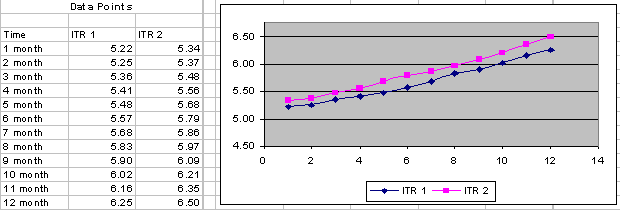
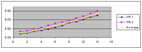
Image: AVG

Average returns the average value between two values. For example, following is a plot of internal transfer rate 1 and internal transfer rate 2, with the average of the two data sets making up the third plot as the average of the two data sets:

ALSO

Also adds a new source to an already calculated operation and repeats this calculation with the result of the previously calculated result and the new source. Also is most likely used in conjunction with the AVG operation code to average an additional data source with the previously averaged values.

For example, the ITR 1 curve and the ITR 2 curve are averaged by using the AVG operation code. In addition, you want to calculate the average between this newly calculated average (comprised of the averaged data set ITR 1 and ITR 2) and the Corp BB curves. This is done by using the ALSO operation code.

(ITR 1 + ITR 2) /2 = Average value

(Average + Corp BB) /2 = Also value

Image: ALSO

The following graph illustrates the ALSO operation code:

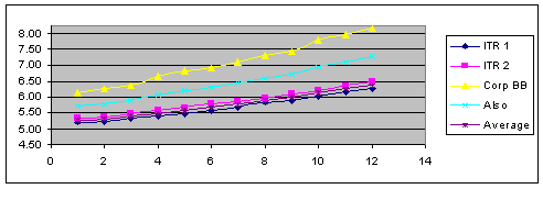
Note: Average represents the average between ITR 1 and ITR 2.Also represents the average between average and Corp BB.

DIFF

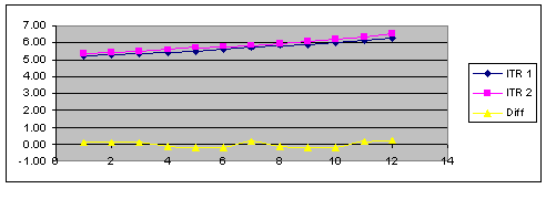
Image: DIFF

This operation code calculates the absolute difference between two yields. DIFF subtracts the lower from the higher value and displays the new value. No negative values can result from this operation. The following graph illustrates the DIFF operation code.

MIN

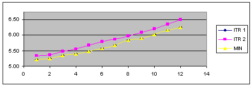
Image: MIN

MIN calculates the absolute minimum value from two sources. This operation code compares two data sets and selects the lowest representative data point between the two data sets. The following graph illustrates the MIN operation code.

MAX

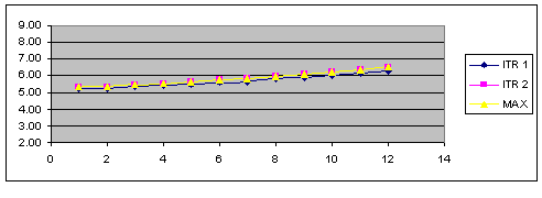
Image: MAX

MAX calculates the absolute maximum value from two sources. This operation code compares two data sets and selects the greatest representative data point between the two data sets. The following graph illustrates the MAX operation code.

SHIFT

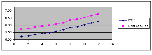
Image: SHIFT

The SHIFT operation code allows the user to apply a basis point shift to an existing data set. The basis point shift is applied to the entire data set. The following graph illustrates the SHIFT operation code.

SHIFT RANGE

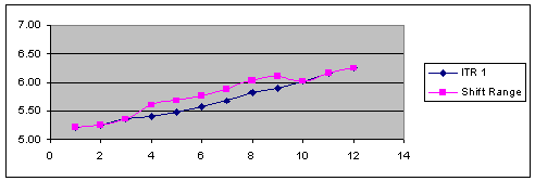
Image: SHIFT RANGE

SHIFT RANGE allows the user to apply a basis point shift to an existing data set that is within a specified time frame. The time frame is specified with a start maturity and an end maturity, which are defined in days, months, or years rather than as actual dates. The following graph illustrates the SHIFT RANGE operation code.

SPLICE

Splice divides an existing curve into a new curve with two or more data sources or types of interpolants.

Note: A curve's interpolant can be spliced only if Global Interpolant isnot selected.

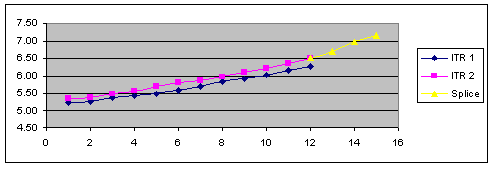
Image: SPLICE

The following graph illustrates the SPLICE operation code.

SUM

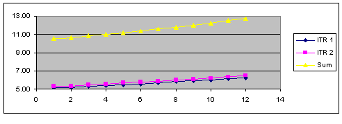
Image: SUM

The SUM operation code adds the data points of two data sets and creates a third data set with the totals. The following graph illustrates the SUM operation code.

Data Source Page

Use the Data Source page (YC_DATA_SRC_PNL) to set up the data source within the system.

Navigation

select Financial Services Industries, then select Interest Rate Environment, then select Dataset Definition, then select Curve Sets, then select Data Source

Image: Data Source page

This example illustrates the fields and controls on the Data Source page. You can find definitions for the fields and controls later on this page.

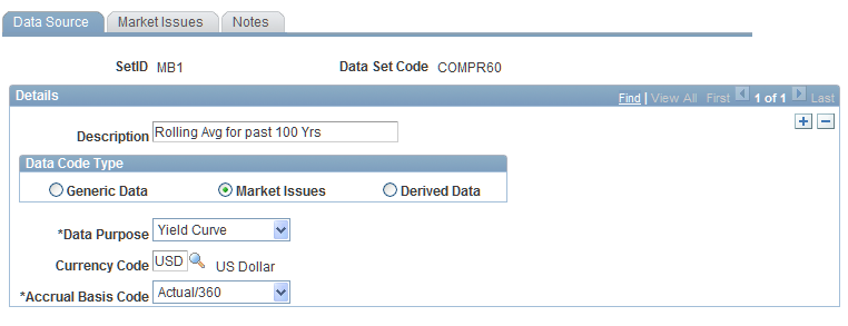
Specify the type of data sets from which you construct the yield curves. Options are:

Generic Data.

The source data is composed of user-defined data. You supply the x-y axis coordinates and units of measure for this data.
Market Issues (default).

The market rate instrument data is assigned to this source data.
Derived Data.

Create your own data from more than one market source. Your choice determines the type of tab that follows the Data Source tab.

Specify the purpose for these data set points. Options are Yield Curve, Commodity, Credit Spread,Foreign Exchange, Volatility, orOther. Specify the currency code and the accrual basis code. Set up the second tab (subsequent Curve Sets page). This tab varies according to the selection in theData Type field.

Data Source Page for Rolling Averages

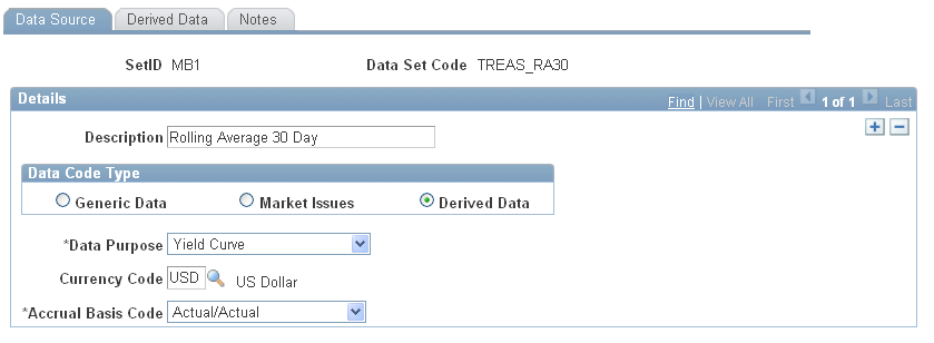
Use Data Source page for rolling averages

Navigation

select Financial Services Industries, then select Interest Rate Environment, then select Dataset Definition, then select Curve Sets, then select Data Source.

Image: Data Source page for rolling averages

This example illustrates the fields and controls on the Data Source page for rolling averages. You can find definitions for the fields and controls later on this page.

Data Code Type

You must select Derived Data for a rolling average curve, meaning that values are calculated or derived from another yield curve.

Note: You first set up a Market Issues curve that sources rates from the market. In the page shot above, there is a Treasury curve called TREAS_SET1 that is populated using daily rates submitted by the U.S. Treasury.

Data Purpose

You must select Yield Curve for a rolling average curve.

Market Issues Page

Image: Market Issues page

This example illustrates the fields and controls on the Market Issues page. You can find definitions for the fields and controls later on this page.

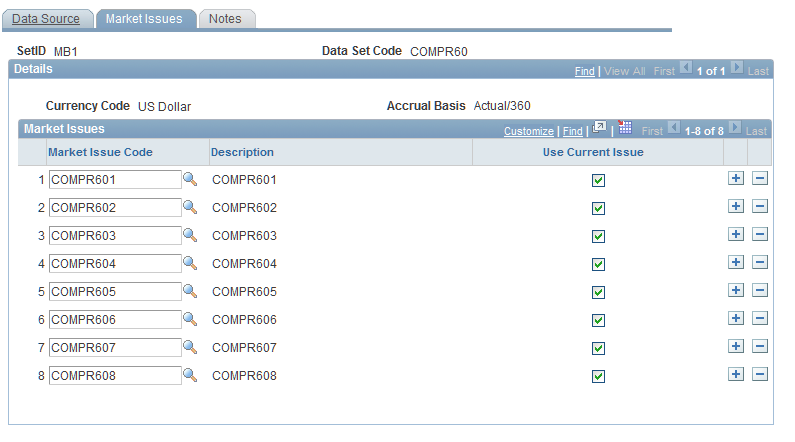
Select a market issue code where you are prompted. Select from codes that you previously set up on the Market Issues page. Specifying a code in this field enables you to create a synthetic curve comprised of numerous market issues that have different attributes and assign those combined market issues to a new data source.

There is a minimum number of data points (market issues that you must select for the curve set definition) to generate unique curve results. This minimum number varies depending on the yield curve interpolation method: 1 for step, 2 for linear, 3 for hermite cubic, and 5 for cubic spline.

Derived Data Page

Use the Derived Data page (YC_COMPST_PNL) to used to create composite curves.

Navigation

select Financial Services Industries, then select Interest Rate Environment, then select Dataset Definition, then select Curve Sets, then select Derived Data

Image: Derived Data page

This example illustrates the fields and controls on the Derived Data page. You can find definitions for the fields and controls later on this page.

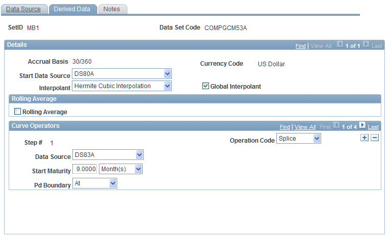
To set up the derived data page, specify the source data that you want to use for this composite curve in the Start Data Source field. Should the construction of data points that you specify require more source data, select an interpolant to use in fitting a curve to the data points. Select theGlobal Interpolant check box to interpolate all the data in the new set in the same manner as the source data that you specify in theStart Data Source field.

If you want to calculate rolling averages based on historic interest rate information, select the Rolling Average check box. This activates two other fields, theLag Frequency andRolling Average Frequency fields that enable you to select dates from previous yield curves.

Next, set up the curve operators. The Step # field indicates the source data that is affected by the chosen operation and helps you keep track of the operations that are performed and the segments of the composite curve that are impacted). Select an operation code to determine operation on the current (and possibly previous) data set that is given in the data source prompt box. Options are:Average, Also, Difference, Max Min, Shift, Shift-Range, Splice, andSum. Depending on the selection, the following fields may appear:

Start Maturity

Valid for the splice and shift-range operation. Defines the maturity at which the new source data or an operation takes effect. You can enter decimal numbers in the following format: 123456.1234. This field is also used to specify the left boundary of a shift-range operation. For example, 1.5 with a corresponding unit of measure of months indicates a start maturity value of 1.5 months. You can enter up to six digits preceding the decimal point and four digits following the decimal point.

Stop Maturity

Defines the maturity at which a shift-range operation ends. If you require multiple shifts over a range, each step can define a new series of start maturity and stop maturity ranges along the constructed composite curve.

Pd Boundary (period boundary)

Use when you splice composite source data. It enables you to specify whether the new source data begins at the start maturity or immediately afterwards.

Basis Points

Enter the number of basis points to shift the curve when the shift operation is chosen. This is a fixed number of basis points across the maturity range that is defined in this step. You may want to create a curve with a rate ramp, rather than a parallel shift. To accomplish this, you need to set up multiple steps with the shift range operation to specify a starting and stopping point for each varied basis point shift for separate segments of the composite curve.

Interpolant

When the Global Interpolant check box is not selected, you can specify the interpolation method for the various steps by using the Interpolant drop down menu. Each step number, or segment of the curve, needs to be defined with an interpolation method. The options are:Cubic Spline,Hermite Cubic, Linear Segments, orStep Function Interpolation.

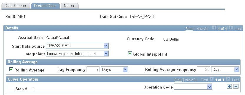
Derived Data Page

Use the Derived Data page

Navigation

select Financial Services Industries, then select Interest Rate Environment, then select Dataset Definition, then select Curve Sets, then select Derived Data.

Image: Derived Data page

This example illustrates the fields and controls on the Derived Data page. You can find definitions for the fields and controls later on this page.

Start Data Source

Specify the source data that you want to use for the composite curve.

For rolling averages, the source data is the Market Issues yield curve that the rolling average calculation is based on. The curve is built prior to building the rolling average curve and generally uses rates sourced from the market. However, it is possible to build a derived curve based on another derived curve.

Interpolant

Specify the interpolation method for the various steps (segment of the curve).

Options are: Cubic Spline, Hermite Cubic, Linear Segments, orStep Function Interpolation. Linear Segments interpolation is the most common method used.

Global Interpolant

Select this check box to use Linear Segments interpolation for the entire curve (you do not have to specify the Operation Code in the Curve Operators section).

Rolling Average

This check box must be selected to perform rolling averages.

Selecting this check box ensures rolling averages are calculated based on historic interest rate information.

Selecting this check box also activates the Lag Frequency andRolling Average Frequency fields.

Lag Frequency

Specify the delay in time that you want your calculation to begin.

The lag frequency shifts the time period that the rolling average is calculated on by the period that you specify. For example, if you set the rolling average frequency to 30 with a 7 day lag frequency, the original calculation changes from: days = t, t-1, t-2, [...] t-30 to days = t-7, t-8, t-9, [...] t-37.

The lag frequency period is not included in the rolling average interest rate calculation unless the value is set to zero.

Rolling Average Frequency

Specify the span of time that is being used to calculate a rolling average.

For example, if February 2002's 8 month rolling average is based on data from April 2001 to November 2001, then March 2002's 8 month rolling average is based on data from May 2001 to December 2001 data.

Generic Data Page

Use the Generic Data page (YC_GENERIC_PNL) to use when creating term structures from generic data sets.

Navigation

select Financial Services Industries, then select Interest Rate Environment, then select Dataset Definition, then select Curve Sets, then select Generic Data

Image: Generic Data page

This example illustrates the fields and controls on the Generic Data page. You can find definitions for the fields and controls later on this page.

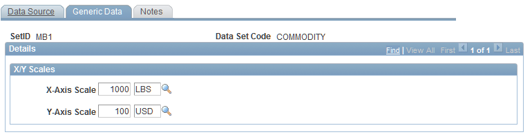
Enter values for the x and y axis. These values are previously set up in PeopleSoft EPM by using the Unit of Measure page. Create generic data sets to provide maximum flexibility for curve generation of desired user defined parameters and data. You provide the data inputs and measures that are needed to define the data set.