18 Offer Optimization

This chapter describes the Promotion and Markdown Optimization and Oracle Retail Offer Optimization Cloud Services. In general, throughout the document the term "Offer Optimization" is used to refer to these two combined services. However, when a specific component is only available in one of these services, the complete service name is used.

Overview

Offer Optimization (OO) is used to determine the optimal pricing recommendations for promotions, markdowns or targeted offers. Promotions and markdowns are at the location level (for example, price zone). Targeted Offers can be specific to each customer and not just to a location. Pricing recommendations contain answers to the following questions: Which items,? When (timing)? and How deep and Who (segments)?. Promotion and Markdown Optimization caters to the retailers who are interested in only promotions and markdowns. Offer Optimization not only provides promotions and markdowns but also targeted offers that are specific to each customer segment. In order to use targeted offers, the retailer must provide customer-linked sales transactions data; to use promotions and markdowns, the retailer does not necessarily have to provide customer-linked sales transaction data.

Certain aspects of promotions, markdowns, and targeted offers are important levers for managing the inventory over the life cycle of the product. The application helps in the following:

• Bring inventory to the desired level, not just during the full-price selling period.

• Maximize the total gross margin amount over the entire product life cycle.

• Assess in-season performance.

• Provide updated recommendations each week. This facilitates decision-making that is based on recent data, including new sales, inventory, price levels, planned promotions, and other relevant data.

• Provide targeted price recommendations at the segment-level.

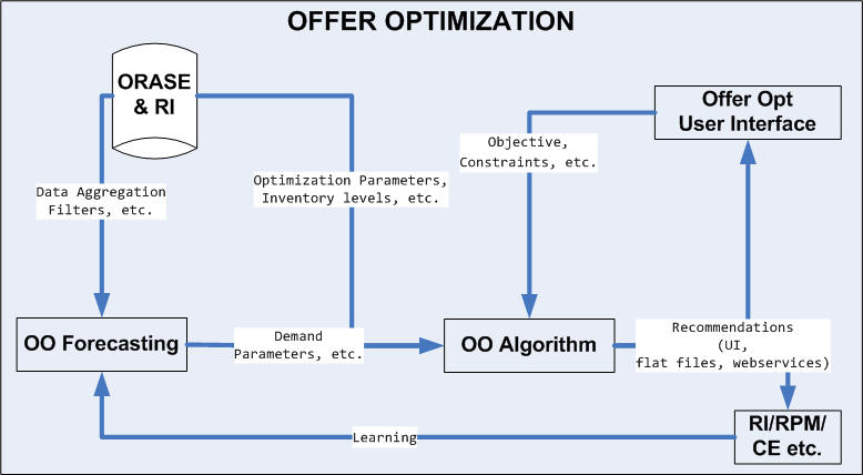
Figure 18-1 shows the conceptual flow of different components in Offer Optimization. ORASE/RI is the core data foundation layer that consumes the retailer data. Offer Optimization Forecasting analyzes historical data to provide the forecasting inputs to the Optimization Algorithm. The Optimization Algorithm obtains inputs such as objectives, budgets, and business rules from the UI, along with optimization parameters from ORASE/RI. The algorithm analyzes the feasible price paths efficiently and generates price recommendations. These recommendations can be viewed in the Offer Optimization UI or can be exported to the price execution systems such as Oracle Retail Price Management (RPM) or Oracle Retail Customer Engagement (CE). In addition, a feedback loop from the price execution systems can helps the OO Forecasting component to determine how the offers are performing and adjust the next set of offers based on the determination. OO supports two kinds of runs, called "ad hoc runs" and "batch runs." Batch runs are scheduled to run automatically at regular intervals (for example, every week). Each batch run, using latest sales data and inventory levels, updates the parameters and budgets and produces the price recommendations. An analyst can review the results and copy the run in order to further accept, reject, or override the price recommendations for each item. Once the analyst finishes the review, the run status can be changed to Reviewed. A reviewed run is sent to the buyer for approval. If the buyer approves the recommendations then the buyer can change the run status to Submitted. This indicates that the price recommendations will be sent to a price execution system such as CE or RPM.

Figure 18-1 Offer Optimization

Offer optimization can be carried out at the configured processing (or run) location, merchandise level, and calendar level. Once the optimization is complete, the recommendations can be generated at a lower level than the processing level, called recommendation levels for merchandise level and location level. The location and merchandise level can be any level in the location hierarchy and merchandise hierarchy, respectively. The usual levels for the run are Price-zone, Department, and Week, and for the recommendation, the levels are Price-zone and Style/Color. If Targeted Offers is available, then the recommendations will also be generated at the Customer-Segment level, along with location and merchandise level. The promotions and markdowns are always at the location and merchandise level.

The optimization considers:

• Optimization at one level below the run's merchandise level. For example, if the run merchandise level is Department, then each optimization job is at the Class level.

• At the configured recommendation merchandise level, the inventory is rolled to the desired recommendation merchandise level. The inventory is aggregated across all the locations to the run's location level.

• Price recommendations are generated at the recommendation level for merchandise, location, and calendar level as well as the customer segment level.

For example, if the run location level is Price-zone, the run merchandise level is Department, the run calendar level is Week, and the recommendation level for merchandise is Style/Color, then the recommendations are generated at the Price-zone, Style/Color, Week, and Segment (when TO is available) levels.

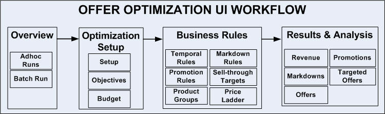
Figure 18-2 shows an overview of the OO UI workflow, which consists of the following:

• Overview. This is the dashboard for the OO runs. In this tab, you can see a list of all existing runs, along with details that describe each run. The list includes runs created by other users, which you can open in read-only mode. You can create a run, copy a run, open a run, or delete a run. The runs overview has three components, Search, Run Status Tiles, and the Table of Runs.

  You can click an existing run or create a new run. Each run is opened in a run tab. The title of the run tab displays "Offer Optimization: <Run ID>". This is the main tab where you can specify the business rules and goals for the run. It provides a series of three stages that you progress through in order to set up, run, and analyze the results of the optimization run.

• Optimization Setup. Used to pick a season, location and department. It is also used to select the objectives and specify the budgets.

• Business Rules. Used to view or change business rules.

• Results and Analysis. Used to view results and override, approve, or revisit prior steps in order to make changes.

Figure 18-2 Offer Optimization UI Workflow

The goal of the implementation is to set up and configure an instance to generate optimal price recommendations that satisfy the retailer's business requirements. The implementation configures the application so that the batch runs complete successfully in a timely fashion and produce valid promotions, markdowns, and forecast recommendations that meet the retailer's requirements. The main implementation tasks involve configuring the following:

• The roles and permissions assigned to users.

• The loading of retailer data.

• The configuration parameters.

• The demand parameters, such as seasonality and price effects, that are used to determine optimal promotion, markdown, and targeted recommendations.

• The business rules that determine constraints that the application takes into account during the optimization process.

Security

User roles are used to set up application user accounts through Oracle Identity Management (OIM). See Oracle Retail Advanced Science Cloud Services Administration Guide for details. Five roles are supported in this application:

• Pricing Administrator

• Pricing Manager

• Pricing Analyst

• Buyer

• Targeted Offer Role

Data Input Requirements

This section provides information about setting up the data that the Offer Optimization application uses to generate optimal price recommendations, including guidelines on the expectations for the data element requested and where it is used. Information about these files can be found in Oracle Retail Insights Cloud Service Suite/Oracle Retail Advanced Science Cloud Services Data Interface.

Hierarchy Data

Hierarchies are part of the core data elements that are used in Offer Optimization, in both the forecasting and optimization modules. The four types of hierarchies are Location Hierarchy, Merchandise Hierarchy, Calendar Hierarchy, and Customer Segments Hierarchy. Hierarchy data is required.

• Location Hierarchy. An example of location hierarchy is: CHAIN ' COUNTRY ' REGION ' DISTRICT ' STORE. The run's optimization location level must match a node in the location hierarchy. For example, you can run the optimization at the District level. Note that the E-com channel can be defined as part of the location hierarchy.

• Merchandise Hierarchy. An example of merchandise hierarchy is as follows: CHAIN ' COMPANY/BANNER 'DIVISION ' DEPARTMENT 'CLASS ' SUBCLASS ' STYLE ' COLOR ' SIZE (SKU). Since Offer Optimization is designed for fashion apparel, it is expected that the you will provide Style and Color through the relevant interfaces. However, if the retailer deals with merchandise such as electronics, that does not necessarily have style or color, the application will work but some of the UI functionality will not be helpful since it is designed primarily for fashion apparel. For example, Custom Rule has the merchandise selectors Class, Subclass, and Style. If no styles are loaded, then the last selector will not be helpful. Further, in such a situation, the recommendation levels will be at SKU level, as other levels will not be meaningful.

• Calendar Hierarchy. This is one of the core hierarchies. The retailer can specify the calendar depending on their business requirements (for example, fiscal calendar).

• Customer Segments Hierarchy. Offer Optimization supports pricing recommendations at the customer segment level. To use this functionality, the retailer must load customer segments. Note that at this time, the Offer Optimization supports only one customer segment group at a time.

Runs in the Offer Optimization can be set up to run at configured levels for location, merchandise, calendar, and customer levels.

• Location Level. The run's location processing level is configurable in RSE_CONFIG, and it is denoted as PRO_LOC_HIER_PROCESSING_LVL. For example, a typical level is Price-zone level.

• Merchandise Level. The run's merchandise processing level is configurable in RSE_CONFIG, and it is denoted as PRO_PROD_HIER_PROCESSING_LVL. For example, a typical level is Style/Color level.

• Calendar Level. The run's calendar processing level is configurable in RSE_CONFIG, and it is denoted as PRO_CAL_HIER_PROCESSING_LVL. For example, a typical level is Week.

• Customer Level. The run's customer processing level is configurable in RSE_CONFIG, and it is denoted as PRO_CUST_HIER_PROCESSING_LVL. For example, a typical level is Segment or Chain (that is, segment-all).

• Setup Level. The run is set up at a level higher than the run's merchandise level. This is configurable in RSE_CONFIG, and it is denoted as PRO_PROD_HIER_RUN_SETUP_LVL. For example, a typical level is Department level.

In this guide, the typical processing levels are generally used as illustration. If necessary, further details will be used to clarify non-typical levels. These levels are also important for the forecasting module since it provides the relevant parameters at the appropriate levels so that it can be consumed by the optimization module.

It is essential that the configuration levels be decided based on the business of the retailer at the time of implementation. These configuration levels dictate how to specify business rules (for example, what is the minimum number of weeks of separation between consecutive markdowns).

Hierarchies are assumed to be set up once for each season and can be revisited whenever it changes. It is expected that the hierarchies do not change from one week to next week within a year (or season). Since hierarchies are core foundational elements any change to hierarchies can be costly and must be planned accordingly. For example, if customer segments are redone, then the parameters must be recalculated. The retailer must plan for such changes as such changes cannot necessarily be completed in the normal weekly batch process or window.

Retail Sales Data

Retail Sales data is a required interface. OO requires you to provide retailer's historical sales data at the desired hierarchy levels. If you want to use the targeted offers, then you must provide the customer-linked transactions sales data. The retailer does not have to provide the data aggregated to the segment-level but must provide the customer ID and customer segment mapping as part of customer segment interface.

Note that the sales returns are handled in the same interface. The returns data identifies the original location where the item was purchased and when it was purchased. This information is useful in returns analysis and in calculating the returns parameters.

When the system is in production, the latest incremental sales data is obtained as part of the batch process.

Historical Promotions

OO requires you to provide any promotions that have occurred in the past. This interface provides the retailer with the ability to specify start and end dates of a promotion event and to specify the Deal Type (for example. BOGO) and Channel (for example, Social). This interface does not allow you to specify which merchandise or locations is part of the promotion. This information is not critical but it can help OO in two ways: identify when the promotions have occurred in the past and learn which future planned promotions are similar to the ones in the past. Historical Promotions are optional.

Competitor Prices

The Competitor Prices interface, which is optional, is used to provide competitor prices. Competitor prices are used to restrict the price recommendations to a certain percent range of the competitor price. For example, if the retailer wants to match the competitor's promotion of 20 percent off but with some tolerance, then this interface allows the retailer to specify the competitor price through the interface. Tolerance is specified as a global parameter in RSE_CONFIG. Note that in this release, the product can support only one competitor price.

Product Attributes

Product attributes interfaces have two components. In the first, the interface expects that Style and Color are loaded as product attributes. W_PROD_ATTR_DS is used for image locations and as well as supporting extended hierarchy (that is, Style and Color). If the retailer wants use extended merchandise hierarchy, then the retailer must populate these interfaces.

In the second interface W_RTL_ITEM_GRP1_DS, product attributes are useful in OO forecasting, particularly for targeted offers. Raw product attributes (for example, fabric, material) can be provided through this interface. Diligent attention must be paid to make sure the attribute values are as clean as possible. For example, COKE vs. COK vs. COEK must be normalized to COKE so that OO does not interpret them as different attributes. It is preferred that the retailer uses W_RTL_ITEM_GRP1_DS, since it can support any number of attributes such as BRAND and the batch load process picks up the attributes added there.

Other Required Interfaces

Additional required interfaces include:

• Seasons. Name of the season with start and end dates.

• Season Periods. Defines which periods belong to the season and provides the ability to define period type as Regular or Clearance. This can include Promotion and Markdown Calendar.

• Season Products. Defines which products are associated with this season.

• Season-Class Markdown Effective Day. Effective day for markdowns in a week.

• Price Ladder. Supports three types of price ladders: Price Point, Percentage Off (Ticket Price) and Percentage Off (Full or Original Price).

• Country Locale. Defines the currency based on the location. The same instance can support multiple currencies. For example, US locations must generate price recommendations (and price-related metrics) in USD and Canadian locations must generate price recommendations (and price-related metrics) in CAD.

• Plan Promotion. Defines future planned promotions. You must specify when (time), which items, and how deep as part of this interface.

Other Optional Interfaces

The interfaces specified in this section are not required. When the retailer provides the necessary required data, the OO Forecasting module generates the demand parameters and supplies it to the Offer Optimization module. However, if the retailer chooses to use their own or another forecasting module, then these interfaces provide a mechanism for the retailer to upload those parameters to Offer Optimization module. These can also be used for proof-of-concept if implementation teams do not have time to go through the full implementation process.

Optimization (useful for proof-of-concept)

• Inventory

• Price Cost

• Optimization Metrics

Forecasting (useful when using own forecasting parameters or for proof-of-concept)

• Baseline

• Price Elasticity

• Return Parameters

• Seasonality

• Model Dates

• Lifecycle Fatigue

• Plan Promotion Lift

Expected Levels for Interfaces

The expected levels for the interfaces are based on the configuration levels specified. Two configuration levels are generally related to hierarchies, recommendation levels and processing levels.

Table 18-1 Configuration: Expected Levels

Data	Configuration Parameters	Customer Segment	Calendar	Merchandise	Location
Optimization Level	Levels at which the optimization process is executed (Units of work)	PRO_CUST_HIER_PROCESSING_LVL	PRO_CAL_HIER_PROCESSING_LVL	PRO_PROD_HIER_PROCESSING_LVL	PRO_LOC_HIER_PROCESSING_LVL
Recommendation Level	Level at which the recommendation results are generated	PRO_OPT_CUST_REC_LVL	PRO_OPT_TIME_REC_LVL	PRO_OPT_MERCH_REC_LVL	PRO_OPT_LOC_REC_LVL

Depending on the above configuration levels, the interface levels expected are as follows:

Table 18-2 Interfaces: Expected Levels

Data	Interface Name	Notes	Customer	Calendar	Merchandise	Location
Season		Range of time periods (e.g., weeks) for the season. This has to match the calendar hierarchy loaded	N/A	N/A	N/A	N/A
Season Period		Periods (e.g., weeks) within a season where the PRO_PROD_HIER_PROCESSING_LVL (e.g., CLASS) is active	N/A	PRO_CAL_HIER_PROCESSING_LVL Date range could span multiple calendar units (i.e. Multiple weeks)	PRO_PROD_HIER_PROCESS-ING_LVL
Season Product		Products that must be included in given selling seasons	N/A	PRO_CAL_HIER_PROCESSING_LVL Date range can span multiple calendar units (i.e. Multiple weeks)	PRO_OPT_MERCH_REC_LVL
Season Product MKDN Day		Day of the week when markdown is taken. This is applicable only when PRO_CAL_HIER_PROCESSING_LVL is week	N/A	N/A	PRO_PROD_HIER_PROCESS-ING_LVL	N/A
Price Ladder	PRO_PRICE_LADDER_STG	Product price ladder	N/A	N/A	PRO_PROD_HIER_PROCESS-ING_LVL	PRO_LOC_HIER_PROCESSING_LVL
Country Locale	PRO_COUNTRY_LOCALE_STG	Defines the specific locale for the location. Provided at the COUNTRY level	N/A	N/A	N/A	PRO_LOC_HIER_PROCESSING_LVL or any hierarchy level higher
Planned Promotion		Planned promotion at PRO_PROD_HIER_PROCESSING_LVL (e.g., CLASS)	N/A	PRO_CAL_HIER_PROCESSING_LVL Date range could span multiple calendar units (i.e. Multiple weeks)	PRO_PROD_HIER_PROCESS-ING_LVL
Plan Promotion Lift		Lift associated to the planned promotion	PRO_CUST_HIER_PROCESSING_LVL	PRO_CAL_HIER_PROCESSING_LVL	PRO_PROD_HIER_PROCESS-ING_LVL	PRO_LOC_HIER_PROCESSING_LVL
Lifecycle Fatigue		Fatigue that is applied to price elasticity and return percentage	PRO_CUST_HIER_PROCESSING_LVL	PRO_CAL_HIER_PROCESSING_LVL	PRO_PROD_HIER_PROCESS-ING_LVL	PRO_LOC_HIER_PROCESSING_LVL
Returns Parameters		Return percentage and lead time	PRO_CUST_HIER_PROCESSING_LVL	N/A	PRO_PROD_HIER_PROCESS-ING_LVL	PRO_LOC_HIER_PROCESSING_LVL
Price Elasticity		Price elasticity	PRO_CUST_HIER_PROCESSING_LVL	N/A	PRO_PROD_HIER_PROCESS-ING_LVL	PRO_LOC_HIER_PROCESSING_LVL
Seasonality		Product seasonalities	PRO_CUST_HIER_PROCESSING_LVL	PRO_CAL_HIER_PROCESSING_LVL	PRO_PROD_HIER_PROCESS-ING_LVL	PRO_LOC_HIER_PROCESSING_LVL
Baseline		Product baseline	PRO_CUST_HIER_PROCESSING_LVL	N/A	PRO_OPT_MERCH_REC_LVL	PRO_LOC_HIER_PROCESSING_LVL
Model Start Dates	PRO_MODEL_DATES_STG	Model start and end date for each product	N/A	PRO_CAL_HIER_PROCESSING_LVL	PRO_OPT_MERCH_REC_LVL	N/A
Optimization Metrics	PRO_SEASON_CURR_OPT_METRIC_STG	Updates (e.g., weekly) for mkdn and promo price, mkdn and promo count and mkdn and periods when item was promoted	N/A	PRO_CAL_HIER_PROCESSING_LVL	SKU level (Style/Color/Size)	Store
Inventory	RSE_INV_PR_LC_WK_A_STG	Inventory available at the start of the period (e.g., week). Inventory is aggregated to the PRO_LOC_HIER_PROCESSING_LVL (e.g., Price Zone)	N/A	Week	SKU level (Style/Color/Size)	Store
Price Cost	RSE_PRICOST_PR_LC_WK_STG	Price cost for the time period (e.g., week)	N/A	Week	SKU level (Style/Color/Size)	Store

Offer Optimization Forecasting

Offer optimization forecasting has two modules, parameter estimation and demand forecasting. Parameter estimation uses the historical data to determine the seasonality, markdown elasticity, promotion elasticity, and promotion lift (or holiday lift) values. Demand forecasting leverages the parameters estimated from historical data and in-season sales data (the base demand is re-estimated on a regular basis as part of batch process) to determine the demand and generate the forecast.

Offer optimization forecasting supports the following features:

• Separate elasticity values for promotions and markdowns

• Customer segment level parameter values for seasonality, elasticity, and traffic lift for promotion and holidays

• The weather effects from historical data period can be incorporated into the estimation of parameters to remove the bias introduces by weather on forecasted sales.

• The ability to execute the following analysis:

  • Day of the week and time of the day profiles

  • Returns analysis

For both parameter estimation and demand forecasting stages, you can adjust the various settings through a configuration table RSE_CONFIG to reflect the business needs of a given retailer. Specifically, you must change the configuration values (if desired) for APPL_CODE = PMO. This code corresponds to OO Forecasting. Based on the settings from RSE_CONFIG a weekly batch job is used generate demand forecasts every week after the weekly data has been updated. Similarly, a batch job can also be used to re-estimate the parameters at specified intervals to reflect the latest sales trends (for example, every six months).

Parameter Estimation

Parameter estimation requires at least 20 months of data. These requirements exist because

• The data from the first 4-6 weeks of the historical period must be removed from the data analysis so that items can be identified that have truly started selling after beginning of historical data period.

• The full life cycle data is required for all fashion/seasonal merchandise introduced during a fiscal year in order to estimate the seasonality curve for merchandise starting in every fiscal month. The least amount of data required is one year plus the typical season length of the merchandise.

Parameter estimation consists of six stages. Each stage has a series of configurable parameters and the corresponding default values. Modify the default values appropriately for each retailer. Populate the parameter values for all stages before starting the run for estimation of demand parameters.

The six stages are:

1. Data preparation. Defines the levels to which data is aggregated on merchandise, location, customer segment, and time dimensions and selects the merchandise and location levels used for parameter estimation.

2. Preprocessing. Filters the historical data and makes the first determination of item eligibility.

3. Elasticity. Determines the price elasticity for markdowns and promotions.

4. Seasonality. Estimates seasonality trends and identifies partitions with reliable seasonality.

5. Promotion lift. Estimates the traffic lift during promotion and holiday events. Corrects the seasonality curves to remove the traffic lift from promotion and holiday events.

6. Output. Generates parameter files in the format required by demand forecasting and offer optimization.

The parameter estimation stage generates markdown elasticity, promotion elasticity, seasonality and promotion lift values. Together they are referred to as demand parameters.

Data Preparation

The data preparation stage determines the aggregation levels on merchandise, location, customer-segment, and time dimensions. The merchandise and location hierarchy levels are used for estimation of demand parameters.

For removing weather effects, an external data feed is used to provide the impact of weather on sales units for weeks included in historical data. During the data aggregation stage, the impact of weather on historical sales units is removed. This ensures that the estimated parameters represent normal weather conditions and historical weather effects do not influence future forecasts.

Data Aggregation

Sales data, inventory data, and returns data are aggregated on the following dimensions.

• Merchandise. User-defined level of aggregation, typically aggregated to Style, Style-Color level.

• Location. User-defined level of aggregation, typically aggregated to Store Cluster/Price zone level.

• Customer Segment. By default, customer segment data is aggregated at two levels, by individual customer segments and Segment-All, which includes all the segments. You do not have an option to select the aggregation level by customer-segment.

• Time. Default aggregation level is by week. You do not have the option to change the aggregation level by time dimension.

Table 18-3 Data Aggregation

Setting Name and Description	Default Value	Range of Values
Data aggregation - Merchandise Level: Level in the merchandise hierarchy at which data is aggregated for sales, inventory and returns	STYLE-COLOR	Merchandise hierarchy level description
Data aggregation - Location Level: Level in the location hierarchy at which data is aggregated for sales inventory and returns	STORE CLUSTER	Location hierarchy level description
Remove weather effect: If impact of weather on merchandise is available as feed then adjust the sales to reflect normal weather	False	True or False

Hierarchy Levels Selection

Select the merchandise and location levels for which Parameter estimation must calculate demand parameters. Parameter estimation calculates demand parameters for the partitions of the levels that are the cross-products of all the levels you select. In the configuration table, select the highest and lowest levels on merchandise and location hierarchy at which parameters must be estimated. For example, if you select Banner and Department for the merchandise levels and Country and Store-Cluster for the location levels, parameter estimation calculates demand parameters for the partitions in Banner/Country, Country/Store Cluster, Division/Country, Division/Store cluster, Department/Country, Department/Store cluster.

Table 18-4 Hierarchy Levels Selection

Setting Name and Description	Default Value	Range of Values
Parameter estimation - Highest Merchandise Level: Choose the highest merchandise level at which parameters are required. Usually this is Company/Banner if there are multiple banners within the company.	BANNER	Merchandise hierarchy level descriptions
Parameter estimation - Lowest Merchandise Level: Choose the lowest merchandise level at which parameters are required. Usually Class/Sub-Class level, there should be enough data volume at this level to estimate demand parameters.	CLASS	Merchandise hierarchy level descriptions
Parameter estimation - Highest Location Level: Choose the highest location level at which parameters are required. Usually this is Chain/Country level.	COUNTRY	Location hierarchy level descriptions
Parameter estimation - Lowest Location Level: Choose the lowest location level at which parameters are required. Usually this is Store Cluster.	STORE CLUSTER	Location hierarchy level description

Data Validation

Once the data preparation stage is complete, prepare data validation report and review it with the customer to confirm the data loaded matches with their expectations. Include the following in the data validation report.

• Summary of merchandise, location, customer segment, calendar hierarchies

• Sales units and amount by year at Chain and Division levels

• Summary metrics by Department-Price zone

• Sales, Inventory and Product count trends by Fiscal week and Fiscal year at Country-Banner level

• For the following data fields Ticket price, sales price, Item cost, Sales units, Sales amount, Inventory

  • Search for negative and null values

  • Significant percent of records with either negative or null values. Flag for review with customer.

Validating data with the customer is key to identifying potential data related problems early on. Investigate any potential data issues and work with the customer to resolve them. This ensures that the following stages are using the appropriate data.

Preprocessing

The Preprocessing stage filters the historical data to produce a subset of data that produces reliable demand parameters. The Preprocessing stage applies filters at the partition and week level. It performs the initial pruning of bad activity data. It does the first stage of determining eligibility and calculates certain values that can later be used in the calculation of elasticity and seasonality parameters.

Data Filters Week Level

Table 18-5 shows the various week level filters used in the Preprocessing stage. These filters are used to remove individual weekly records of data that do not meet the requirement defined as specified for each filter.

Table 18-5 Data Filters Week Level

Filter Name and Description	Default Value	Range of Values
Store count greater than 0 - used to filter activities with null or zero store count.	False	True or False
SKU store count greater than 0 - used to filter activities with null or zero sku store count.	False	True or False
Inventory data present - this check box is used to indicate that the inventory data is thought to be reliable. If inventory data is thought to be reliable, then Preprocessing and RawAP will use inventory data for filtering and other calculations. If inventory data is thought to be unreliable, then it is ignored.	True	True or False
Sales unit threshold - used to filter sales unit activities with sales units below threshold values.	1	Greater than or equal to 1.
Inventory threshold - used to filter inventory activities with inventory units be-low threshold values.	1	Greater than or equal to 0.
Life cycle sell thru % - the item start and end dates are calculated using per-centage sell through. The start date is the date when Life cycle sell through % (Start) is reached. The end date is the date when Life cycle sell through % (End) is reached. Life cycle sell through % (Start) is expressed relative to 0% so entering 2 means that the start date is when 2% of total sales has been achieved. Life cycle sell through % (End) is expressed relative to 100% so entering 2 means that the end date is when (100-2)% i.e., 98%, of total sales has been achieved.	Start: 2.0 End: 2.0	Start: greater than or equal to 0; less than or equal to 50. End: greater than or equal to 0; less than or equal to 50.
Relative price - relative price thresholds are used to filter out item weeks with a ratio of sales price to maximum ticket price that fall outside the specified range for the start date and the end date.	Start: 0.2 End: 1.0	Start: greater than 0. End: greater than the start value.

Partition Filters

These filters are used to exclude all the weekly records from a Merchandise-Location-Customer segment partition at the aggregation level, for partitions with values that do not meet the requirement specified for each filter, as described below.

Table 18-6 Partition Filters

Filter Name and Description	Default Value	Range of Values
Minimum number of eligible weeks - a certain number of weeks are necessary in order to determine item eligibility.	6	Greater than 0.
Minimum season (weeks) - a certain season length (the number of weeks between the first and last activity) is required in order to determine item eligibility.	6	Greater than 0.
Minimum sales units - the total number of units sold must be at least this value.	10	Greater than 0.
Fraction of eligible weeks - the percentage of eligible weeks, expressed as a fraction of the season length. The season length is the number of weeks between the start and end dates. (See Life cycle sell thru % above.)	0.6	Greater than 0.0; less than or equal to 1.0.

Elasticity

The Elasticity stage determines the promotion and markdown elasticity values at the selected levels in the merchandise and location hierarchy. For a given merchandise and location hierarchy level, this stage also determines the elasticity value by customer segment.

In this stage, parameters must be set for

• Additional data filtering to reduce the noise in the elasticity estimation

• Identifying markdowns weeks

• Identifying promotion weeks

• Reliability thresholds for elasticity estimation

• Transformation of elasticity values

Data Filters Weekly

Additional data filters are applied during the estimation of elasticity. These filters are used to reduce the noise from very deep price cuts or price cuts towards the end of life. An option is also available to the limit the data used for elasticity estimation.

Table 18-7 Data Filters Weekly

Filter Name and Description	Default Value	Range of Values
Relative price - used to filter out item-weeks with a ratio of sales price to maximum ticket price that falls outside the specified range.	Low: 0.2 High: 1.0	Greater than or equal to 0.
Relative inventory - the upper and lower bounds for the value for inventory relative to maximum inventory.	Low: 0.2 High: 1.0	Greater than or equal to 0.
Range filter - used to eliminate unreliable data using start date and end date for the period. Both the start date and the end date are Null by default. A Null value means that the field is not used in the filter. One or both of the fields can have a value of Null. If both of the fields are Null, then the data is not filtered.	Start date: Null End date: Null

Markdowns

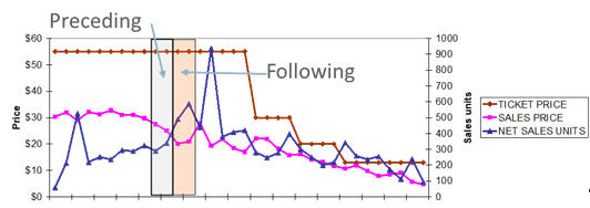
The parameters described below are used to identify markdowns in the aggregated weekly sales data. During a markdown window, the application is interested in a drop in prices from the preceding window to the following window. During a promotion, the application is looking for similar prices during preceding and following window but a drop in prices during promotion window. Similar parameters are used to identify Promotions as well.

Figure 18-3 Markdowns

Time window defines the weeks before and after the markdown. The preceding weeks value is the number of weeks before the markdown occurred. The following weeks value is the number of weeks after the markdown and includes the week of the markdown. A week is a calendar week. A time window that satisfies all the markdown parameter settings is classified as a markdown window.

Minimum eligible weeks is the minimum of the actual number of weeks in the Time Window that have data. The Time Window is in calendar weeks, and not every calendar week actually has sales data. So the actual number of weeks with data that are within the Time Window can actually be smaller than the Time Window.

Maximum deviation is the deviation of the sales price in the weeks before and after the markdown. Provides stability on the variance.

Min Markdown depth is the drop in average sales price from preceding weeks to the following weeks is higher than this threshold value. Markdown depth = 1- (Avg Price following weeks/Avg Price preceeding weeks). In other words, this parameter controls how much of a price decrease is required in order for the price decrease to count as a markdown.

Table 18-8 Markdown Parameters

Name and Description	Default Value	Range of Values
Time Window	Preceding: 2 Following: 2	1–3 1–3
Eligible Weeks	Preceding: 2 Following: 2	1–3 1–3
Maximum Deviation	Preceding: 0.1 Following: 0.1	0–1 0–1
Min Markdown Depth	0.1	0–1
Use Ticket Price: Both Ticket price and sales price values from the preceding and following weeks satisfy min markdown depth criteria.	False	True or False

Promotion One Week

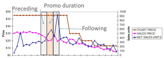
For identifying promotions, a few additional parameters are defined below in addition to Time window, Eligible weeks, and maximum deviation, which are defined above.

Figure 18-4 Promotion

Min Promotion depth is the drop in average sales price during the week of promotion compared to preceding/following weeks. In other words, this parameter controls how much of a price decrease is required in order for the price decrease to count as a promotion.Time window defines the weeks before promotion, during promotions, and after the promotion. The preceding weeks value is the number of weeks before the markdown occurred. The following weeks value is the number of weeks after the markdown and includes the week of the markdown. A week is a calendar week. Time window that satisfies all the promotion parameter settings is classified as a promotion window.Promotion depth = 1- (Avg. Price during promotion weeks/ Avg. price during preceding and following weeks). Time Window - Promo duration: Duration of the promotion event, this is set to 1 for 1-week promotion. Max deviation - Preceding/Following: Avg. price deviation across preceding and following weeks must be less than this threshold. This ensures that the sales price is similar in the weeks before and after the promotion.

Table 18-9 Promotion Parameters

Name and Description	Default Value	Range of Values
Time Window	Preceding: 1 Following: 1 Promo Duration: 1	1–3 1–3 1
Eligible Weeks	Preceding: 1 Following: 1	1–3 1–3
Maximum Deviation	Preceding: 0.1 Following: 0.1 Preceding/Following: 0.1	0–1 0–1 0–1
Min Promotion Depth	0.1	0–1

Promotion Two Week

Promotion duration parameter is set to 2 for identifying two week promotions. Promotion parameters for one week and two week promotions can be set to different values.

Table 18-10 Promotion Two Weeks

Name and Description	Default Value	Range of Values
Time Window	Preceding: 1 Following: 1 Promo Duration: 2	1–3 1–3 2
Eligible Weeks	Preceding: 1 Following: 1	1–3 1–3
Maximum Deviation	Preceding: 0.1 Following: 0.1 Preceding/Following: 0.1	0–1 0–1 0–1
Min Promotion Depth	0.1	0–1

Reliability Settings

Determine the partitions with reliable elasticity values.

Table 18-11 Reliability Settings

Name and Description	Default Value	Range of Values
Outlier threshold: Percentile threshold for removing outlier data points from elasticity estimation. Eg., Threshold is set to X%, Top X Percentile and Bottom X percentile sales ratio and price ratio data points are excluded from elasticity estimation.	0.05	0–0.05
Eligible items threshold - Elasticity	25	Greater than 1.
Std. Error threshold	0.3	0–1

Transformation

Transform the elasticity values obtained after the pruning based on reliability to cap the very low or very high elasticity values. The transformation settings also enable the user to shift the elasticity values to a desired range.

Table 18-12 Transformation

Name and Description	Default Value	Range of Values
Transform Percentile - Low	0.1	0–1
Transform Percentile - High	0.9	0–1
Elasticity range - Min: Select a value closer to the transform percentile - Low and higher than 1.2	1.3	Greater than 1.
Elasticity range - Max: Select a value closer to the transform percentile - high.	2.8	Greater than elasticity range–min.

Seasonality

The Seasonality stage determines the seasonality values at the selected levels in the merchandise and location hierarchy. For a given merchandise and location hierarchy level, this stage also determines the seasonality value by customer segment.

In this stage, parameters must be set for

• Seasonality curve set up

• Reliability filters

Seasonality Curve Setup

The Seasonality Curve Setup stage determines the season codes used for building seasonality curves, length of the seasonality curve, item count threshold, padding curve weight, and seasonality coverage of the final curves.

Season codes create additional partitioning in the dataset by introducing a time dimension. This stage can be used to partition seasonality curves by fiscal start month, fiscal start week, for example, Partition the Class-Store cluster-Customer segment data based on the merchandise time of introduction. Group merchandise based on the fiscal month of the start date. This ensures items starting in the same month receive the same season code. Weekly curves are useful for modeling short life cycle merchandise, while monthly curves are useful for medium to long life cycle curves.

Length of the seasonality curve: Seasonality curves are generated for 52 weeks. They can also be generated for longer duration if the merchandise life cycle length is longer. This also increases the duration of historical data required to prepare the seasonality curves.

Actual sales for a given merchandise-location-customer segment-Start month can be present for less than 52 weeks. To generate a curve for the entire 52 weeks duration, a padding curve is used.

Padding curve: The padding seasonality curve is determined by creating a basic curve for the highest merchandise/location partition. The final seasonality curve is calculated as weight * padding curve + (1 - weight) * seasonality curve.

Table 18-13 Seasonality Curve Setup

Name and Description	Default Value	Range of Values
Curve Type: Determines the duration of time partition based on fiscal week or fiscal month.	Monthly	Monthly or Weekly
Basic Curve: Basic curves are generated by ignoring the partitioning on time dimension for a given merchandise-location-customer segment partition.	True	True or False
Seasonality curve length: Determines the length of the final seasonality curves for regular (non-basic) season codes. The length from the start determines how many weeks after the start date are in the curve.	52	Greater than or equal to 6.
Eligible items threshold: The minimum number of items that a Merchandise Hierarchy/Location Hierarchy/Customer Segment/Season Code partition must contain so that Raw-AP can produce a seasonality curve for the partition.	5	Greater than or equal to 1.
Padding curve weight: The value used in determining the final seasonality curve.	0.4	Greater than 0.0; less than 1.0.
Seasonality Coverage: First Fiscal year	Latest fiscal year with historical data	Greater than or equal to 2018
Seasonality coverage: Last fiscal year	Latest fiscal year with historical data + 2.	Greater than or equal to 2020.

Reliability Filters

The filters in this stage are used to identify reliable seasonality curves based on the number of items in the partition, average sales volume, and season length threshold.

Table 18-14 Reliability Filters

Name and Description	Default Value	Range of Values
Keep top level curves: All the highest level curves are kept, regardless of threshold values.	True	True or False
Prune curves with missing dates: Pruning of basic curves with missing dates is permitted.	True	True or False
Eligible items threshold: Partitions with fewer numbers of eligible items than the threshold value are removed. Eligibility is defined during preprocessing.	5	Greater than or equal to 0.0.
Average weekly sales threshold: Partitions with average weekly sales below the threshold are removed. Weekly sales are the sum of all sales for all activities for a given week.	25	Greater than or equal to o.
Raw seasonality length threshold: Curves can be discarded when the number of weeks from the first non-zero seasonality value to the last non-zero seasonality value is less than the threshold. In the seasonality stage, it is possible that many seasonality values of zero have been added to the curves. Note that basic season codes have a length of 53, so picking a value greater than 53 will prune out any basic season codes. Seasonality curves before padding are referred to as raw seasonality curves.	10	Greater than or equal to 0.

Promotion

The promotion stage determines the traffic lift value associated with promotions and holiday events at the selected levels in the merchandise and location hierarchy. For a given merchandise and location hierarchy level, this stage also determines the promotion lift value by customer segment. A list of holidays and promotions, along with event start date and end date, is sent as a data feed.

In this stage, parameters must be set for determining the baseline to be used for estimation of lift values, Outlier threshold, min lift value. and max lift value.

Table 18-15 Promotion

Name and Description	Default Value	Range of Values
Baseline: The baseline type determines how to smooth the seasonality curve. If you select the linear option, parameter estimation looks at event effective start date and event effective end date and draws a straight line between them. Effective start date is the weekend prior to the event start date and effective end date is the second weekend after the event end date.	Linear	Linear, Min, or Max.
Outlier percentile: Very high lift values are flagged.	0.05	0–1
Lift value -High: Lift values flagged as outliers are capped to outlier percentile lift value.	True	True or False
Lift value-min; Sets the threshold for min lift value. Any promotions with lift value lower than this threshold are not assigned any lift value.	1.05	Greater than or equal to 1.

Output

The settings in the Output stage determine the level at which parameters are exported to Offer Optimization. Offer Optimization typically expects the parameters at the lowest level of estimation. For example, Offer Optimization expects the demand parameters at Class-Store cluster level. Use escalation to fill in the parameters missing at Class-Store level. The Output stage escalates on location hierarchy first and then on merchandise hierarchy.

Table 18-16 Output

Name and Description	Default Value	Range of Values
Parameter-Merchandise hierarchy level	CLASS	Merchandise level description
Parameter-Location hierarchy level	STORE–CLUSTER	Location level description

Run the parameter estimation by starting the batch process during the implementation phase. Details on the batch processing are covered in a separate section. PMO_LOG_TBL can be used to track the progress of the run. Once the parameter estimation is complete, review the parameter values using the Innovation Workbench. Perform the following checks after each stage in the parameter estimation is complete.

Elasticity (pmo_elasticity_parameters)

• Histogram of elasticity values, promotion vs markdown: Distribution of elasticity values follows the expected trend. Typically follow a normal distribution around the median elasticity value.

• Elasticity escalation: Percentage of partitions receiving elasticity values from higher level.

Seasonality (pmo_seasonality_parameters; pmo_seasonality_curve_tbl)

• Review number of partitions impacted by reliability filters:

• Visually check the top level seasonality curves

• Seasonality escalation: Percentage of partitions receiving elasticity values from higher levels.

Promotion lift (pmo_promtoion_lift)

• Plot histogram of promotion lift values by event and compare across segments.

Day Level and Returns Metrics

This section covers the settings used for determining day of the week profiles, time of the day profiles, return rate, and average time to return.

Day of the Week Profiles

Day of the week profiles determine the relative sales strength across various days in a given week. These profiles are used to spread the forecasted demand to the day level. In order to capture the variation across merchandise, location, segment, and calendar dimension, the configuration on each of the four dimensions is supported. In the current version, you can chose two configurable levels for estimating day of the week profiles. Level 1 corresponds to the level at which profiles are to be estimated, and Level 2 profiles are only used when Level 1 profiles are not available.

Table 18-17 Day of the Week Profiles

Name and Description	Default Value	Range of Values
Merchandise level 1	DEPARTMENT	Merchandise level description
Location level 1	STORE CLUSTER	Location level description
Customer segment level 1	BOTH	SEGMENT, SEGMENT ALL, BOTH
Calendar level 1: when calendar level is set to year, use the data from the most recent 52-week period.	YEAR	Calendar level description
Merchandise level 2	DIVISION	Merchandise level description
Location level 2	COUNTRY	Location level description
Customer segment level 2	BOTH	SEGMENT, SEG-MENT ALL, BOTH
Calendar level 2: when calendar level is set to year, use the data from the most recent 52-week period.	YEAR	Calendar level description
Std. Deviation threshold: This threshold value is used to exclude days with very high or very low sales values. Threshold value of 1 indicates only weeks with sales value between median - standard deviation and median+ standard deviation are used for estimating the day of the week profiles.	1	0.5–3
Sampling %: This setting determines the number of weeks used. Using a value of 25% implies the use of only 1/4th of the available weeks in the calendar level to determine the profiles. Whenever sampling % is less than 100%, selected weeks are spread uniformly over the calendar period.	100%	10%; 20%; 25%; 30%; 50%; 100%
Sales threshold: Total sales from the merchandise, location, segment and calendar partition must be higher than this threshold value for the partition to be eligible for estimation of day of the week profile.	1000	Greater than 100.

Time of Day Profiles

Time of the day profiles determine the relative sales strength across various day parts in a given day. Each day is divided into multiple day parts defined by start time and end time and day part sequence. Day part sequence defines the beginning day part and ending day part. These profiles are used to understand the customer purchasing behavior during different times of the day. Level 1 corresponds to the level at which profiles are to be estimated, and Level 2 profiles are only used when Level 1 profiles are not available.

Table 18-18 Time of Day Profiles

Name and Description	Default Value	Range of Values
Merchandise level 1	DEPARTMENT	Merchandise level description
Location level 1	STORE CLUSTER	Location level description
Customer segment level 1	BOTH	SEGMENT, SEGMENT ALL, BOTH
Calendar level 1: when calendar level is set to year, use the data from the most recent 52-week period.	YEAR	Calendar level description
Merchandise level 2	DIVISION	Merchandise level description
Location level 2	COUNTRY	Location level description
Customer segment level 2	BOTH	SEGMENT, SEGMENT ALL, BOTH
Calendar level 2: when calendar level is set to year, use the data from the most recent 52-week period.	YEAR	Calendar level description
Std. Deviation threshold: This threshold value is used to exclude days with very high or very low sales values. Threshold value of 1 indicates only weeks with sales value between median - standard deviation and median+ standard deviation are used for estimating the day of the week profiles.	1	0.5–3
Sampling %: This setting determines the number of weeks used. Using a value of 25% implies the use of only 1/4th of the available weeks in the calendar level to determine the profiles. Whenever sampling % is less than 100%, selected weeks are spread uniformly over the calendar period.	100%	10%; 20%; 25%; 30%; 50%; 100%
Sales threshold: Total sales from the merchandise, location, segment and calendar partition must be higher than this threshold value for the partition to be eligible for estimation of time of day profile.	1000	Greater than 100.

Returns Metrics

For returns, the return rate and average time to return metrics are determined at two levels that are configurable. Level 1 corresponds to the level at which profiles are to be estimated, and Level 2 profiles are only used when Level 1 profiles are not available.

Return rate determines the percentage of total sales units that are returned. Average time to return determines the average number of days between the purchase date and return date of the merchandise. For estimating the average time to return, the original transaction ID information must be included, along with the transaction ID corresponding to a return.

Table 18-19 Returns Metrics

Name and Description	Default Value	Range of Values
Merchandise level 1	DEPARTMENT	Merchandise level description
Location level 1	STORE CLUSTER	Location level description
Customer segment level 1	BOTH	SEGMENT, SEGMENT ALL, BOTH
Calendar level 1: when calendar level is set to year, use the data from the most recent 52-week period.	YEAR	Calendar level description
Merchandise level 2	DIVISION	Merchandise level description
Location level 2	COUNTRY	Location level description
Customer segment level 2	BOTH	SEGMENT, SEGMENT ALL, BOTH
Calendar level 2: when calendar level is set to year, use the data from the most recent 52-week period.	YEAR	Calendar level description
Sales threshold: Total sales from the merchandise, location, segment and calendar partition must be higher than this threshold value for the partition to be eligible for estimation of returns metrics.	1000	Greater than 100.

Batch Processing

Batch processing is set to run at fixed intervals. All the settings set by the implementation team must be used for subsequent parameter estimation runs unless changed by the users before the next batch run.

During the initial implementation, some of the settings are determined by running the parameter estimation stage iteratively. In order to run a specific stage within parameter estimation process, the following option executing batch process on demand is provided.

A batch process can be executed on demand through the interface file pro_run_execution.txt with the following fields. Once the parameter estimation is started with this process, all the stages must be completed through this interface.

Action. The following set of predefined actions are available to the user. EXECUTE will run the specific stage. APPROVE is used to approve the results/output. EXPORT is used to export the parameters.

Stage. Specific stages for which the action is requested. PREPROCESSING, ELASTICITY, SEASONALITY, PROMOTIONS, OUTPUT. Multiple stages can be run at the same time through the batch process by leveraging this methodology.

pro_run_execution.txt: Here is Sample data:

• ACTION|STAGE

• EXECUTE|PREPROCESSING

• EXECUTE|ELASTICITY

• EXECUTE|SEASONALITY

• EXECUTE|PROMOTIONS

• EXECUTE|OUTPUT

• EXPORT|PARAMETERS

The sample text file executes pre-processing, elasticity stages, seasonality, promotions, outputs stages, and exports the parameters for demand forecasting. You can run a particular stage multiple times in order to refine the settings.

Demand Forecasting

The following multiplicative demand model is used as follows:

Demand = Base demand* Seasonality *Price effect* Promotion Lift*Store count

Base demand is updated in season every week at the Optimization recommendation level, Style Color-Store cluster-Customer segment level. Demand forecasting leverages the parameters estimated from historical data and in-season sales data to generate a demand forecast. Elasticity for determining price effect is assigned using merchandise and location hierarchy. For assigning seasonality curve and promotion lift, the start date is required to determine the right partition on time dimension in addition to merchandise and location hierarchy. Demand forecasting set up involves configuration for start date and demand strategy.

Demand forecasting stage leverages the parameters estimated from historical data and in-season sales data to generate a demand forecast. Demand forecast values along with historical parameters are sent to Offer Optimization for generating optimal price recommendations and targeted offers.

In this stage, the following parameters must be set by the user to determine the model start date, season code and demand model settings.

Table 18-20 Demand Forecasting

Name and Description	Default Value	Range of Values
Start date - sell thru %: The earliest week ending date when a Style-Color - Store Cluster combination achieves 2% sell thru is used to determine its start date. The start date is used to determine the seasonality curve assigned to a style color - store cluster combination.	2%	0%–5%
Start date - max weeks from first sale: After the first sale date if the 2% sell thru is not achieved before this threshold then first sale date + max weeks from first sale is used to define the start date	3	1–5
Seasonality - Curve type: This setting must match the Curve type setting in the parameter estimation stage.	Monthly	Monthly or Weekly
Seasonality - Max weeks from start: This setting is used to switch from a fashion curve to a basic curve if an item lives longer than expected.	42	Greater than 35.
Demand strategy: Select the demand strategy to be used in forecasting demand. Genuine Bayesian works well especially when rate of sale is lower. Use Average when rate of sale is very high typically more than 20.	Genuine Bayesian	Genuine Bayesian or Average
Demand Interval: Number of in-season weeks to be used for demand forecast-ing.0 implies the use of entire history from current season to generate the demand forecast. For Genuine Bayesian, use entire history or very large number of weeks from in-season data. For Average, use 2-4 weeks, since average is used in high rate of sale scenarios; using more recent weeks of data is preferred.	0	0–5
Alpha: smoothing parameter. This parameter determines how quickly the weights decay for past weeks in-season data.	0.7	0–1

Offer Optimization Science

This section describes the business rules that are available and the science behind the optimization algorithms used in the Offer Optimization application. It does not provide all the details of the algorithm. However, it does provide some guidance so that you can troubleshoot and resolve issues quickly during an implementation.

Business Rules

The implementation of Offer Optimization is determined by a retailer's individual business requirements. A complete and accurate configuration of business rules is essential to the accuracy and success of the recommendations and forecasts.

Some of the business requirements or rules include:

• The retailer's pricing strategy for promotions, markdowns, and targeted offers. Does the retailer want to maximize the revenue or profit margin?

• The level of the merchandise hierarchy and of the location hierarchy at which the sales data will be provided.

• The level of the merchandise and location hierarchies at which the item is defined.

• The day of the week that markdowns are effective. Typical start and end date for promotions during a week.

• Whether markdowns are effective on the same day or different days for all departments.

• Whether promotions, budget, and distribution center data will be included in the data feed.

• How eligible items (items to be processed by OO in a given week) are defined (for example, if an item exists in the most recent sales data feed and has a threshold number of units on hand).

• The kinds of inventory that must be considered by the batch process for optimization.

It is essential that considerable time be spent on understanding the business rules so that the global defaults can be populated in RSE_CONFIG with APPL_CODE ='PRO' and so most of the departments will not require further tweaking of the batch runs or for ad hoc runs. The configuration that must be created in conjunction with the business requirements are:

Table 18-21 Business Rules

PARAM_NAME	PARAM_VALUE	DESCR
DEFAULT_APPL_USER	OO_BATCH_USR	User identifier to be used for batch activities that require user tracking.
PRO_PROD_HIER_TYPE	3	The hierarchy ID to use for the product (Installation configuration).
PRO_LOC_HIER_TYPE	2	The hierarchy ID to use for the location (Installation configuration).
PRO_CAL_HIER_TYPE	11	The hierarchy ID to use for the calendar (Installation configuration).
PRO_CUSTSEG_HIER_TYPE	4	The hierarchy ID to use for the customer segments (Installation configuration).
PRO_CAL_HIER_PROCESSING_LVL	4	The calendar hierarchy level at which PRO will define RUNs for optimization.
PRO_PROD_HIER_RUN_SETUP_LVL	4	The merchandise hierarchy level at which PRO will setup/create RUNs.
PRO_PROD_HIER_PROCESSING_LVL	5	The merchandise hierarchy level at which PRO will optimize RUNs.
PRO_LOC_HIER_PROCESSING_LVL	4	The location hierarchy level at which PRO will define RUNs for optimization.
PRO_CUST_HIER_PROCESSING_LVL	2	Default customer segment level at which PRO will define RUNs for optimization.
PRO_OPT_LOC_REC_LVL	4	Default location level at which price recommendations will be generated (Store).
PRO_OPT_CUST_REC_LVL	1	Default customer segment level at which price recommendations will be generated (whole population).
PRO_OPT_TIME_REC_LVL	4	Default calendar level at which price recommendations will be generated (week).
PRO_OPT_MERCH_REC_LVL	9	Default merchandise level at which price recommendations will be generated (STYLE-COLOR).
PRO_OPT_MECH_REC	NONE	Default targeted offer mechanics for which price recommendations will be generated.
PRO_OPT_MKTG_REC	NONE	Default targeted offer marketing aspect for which price recommendations will be generated.
PRO_SALVAGE_VALUE	0	Salvage value is the value of the product after the season ends. default value is 0.
PRO_TR_NO_TOUCH_AFTER_LANDING	0	Default no touch after landing (2 weeks).
PRO_TR_LENGTH_OF_PROMOTIONS	0.6	Default length of promotion as a percentage of the whole season.
PRO_TR_MAX_LENGTH_OF_PROMOTION	1	Default maximum length (weeks) of a promotion .
PRO_TR_LENGTH_OF_MKDN	0.4	Default length of markdown as a percentage of the whole season.
PRO_TR_NO_TOUCH_END_LIFE	0	Default no touch at the end of life (1.5 weeks).
PRO_PR_FIRST_PROMO_MIN_DISC_PCT	0	Default minimum discount percentage for the first promotion.
PRO_PR_FIRST_PROMO_MAX_DISC_PCT	1	Default maximum discount percentage for the first promotion.
PRO_PR_OTHER_PROMO_MIN_DISC_PCT	0	Default minimum discount percentage for promotions other than the first one.
PRO_PR_OTHER_PROMO_MAX_DISC_PCT	1	Default maximum discount percentage for promotions other than the first one.
PRO_PR_MIN_TIME_BETWEEN_PROMOS	1	Default minimum time separation between any two consecutive promotions (1 week).
PRO_PR_PROMO_START_DAY	MONDAY	Day of the week promotions start
PRO_PR_PROMO_END_DAY	SUNDAY	Day of the week promotions end
PRO_PR_DAY1_WGT	0.14	Promotion weight for day 1 of the week
PRO_PR_DAY2_WGT	0.14	Promotion weight for day 2 of the week
PRO_PR_DAY3_WGT	0.14	Promotion weight for day 3 of the week
PRO_PR_DAY4_WGT	0.14	Promotion weight for day 4 of the week
PRO_PR_DAY5_WGT	0.14	Promotion weight for day 5 of the week
PRO_PR_DAY6_WGT	0.15	Promotion weight for day 6 of the week
PRO_PR_DAY7_WGT	0.15	Promotion weight for day 7 of the week
PRO_MR_FIRST_MKDN_MIN_DISC_PCT	0	Default minimum discount percentage for the first markdown.
PRO_MR_FIRST_MKDN_MAX_DISC_PCT	1	Default maximum discount percentage for the first markdown.
PRO_MR_OTHER_MKDN_MIN_DISC_PCT	0	Default minimum discount percentage for markdowns other than the first one.
PRO_MR_OTHER_MKDN_MAX_DISC_PCT	1	Default maximum discount percentage for markdowns other than the first one.
PRO_MR_MIN_TIME_BETWEEN_MKDN	1	Default minimum time separation between any two consecutive markdowns (1 week).
PRO_MR_MKDN_START_DAY	MONDAY	Day of the week markdown start
PRO_MR_MKDN_END_DAY	SUNDAY	Day of the week markdown end
PRO_MR_DAY1_WGT	0.14	Markdown weight for day 1 of the week
PRO_MR_DAY2_WGT	0.14	Markdown weight for day 2 of the week
PRO_MR_DAY3_WGT	0.14	Markdown weight for day 3 of the week
PRO_MR_DAY4_WGT	0.14	Markdown weight for day 4 of the week
PRO_MR_DAY5_WGT	0.14	Markdown weight for day 5 of the week
PRO_MR_DAY6_WGT	0.15	Markdown weight for day 6 of the week
PRO_MR_DAY7_WGT	0.15	Markdown weight for day 7 of the week
PRO_ST_END_REGULAR_SEASON	0.15	Default percentage of sell-through for each individual product at end of regular periods.
PRO_ST_END_CLEARANCE_SEASON	0.85	Default percentage of sell-through for each individual product at end of clearance season.
PRO_ST_TGT_TYPE	HARD	individual product.
PRO_ST_HARD_TGT_FLG	Y	Default value for sell-through hard target flag.
PRO_DFLT_RETURN_PCT	0.01	Default percentage of sales returned.
PRO_DFLT_RETURN_LEAD_TIME	2	Default return lead time in weeks (time when the return happens after the pur-chase is made).
PRO_PR_MIN_COST	Y	Promotions recommendations cannot be lower than the cost of the product.
PRO_MR_MIN_COST	Y	Markdown recommendations cannot be lower than the cost of the product.
PRO_BASE_INITIAL_BUDGET	9999999	Initial Budget for Base Scenarios.
PRO_SEAS_CURVE_WEEKS_SWITCH	42	Seasonality Curve.
PRO_OFFERMAX	3	Maximum number of offers for segment in a given time period.
PRO_LOWRR	0.20	threshold value used to pick at least one low redemption rate offer for a segment and given time period.
PRO_HIGHRR	0.80	High Redemption Rate. This is a threshold value used to pick at least one high redemption offer for a given segment and given time period.
PRO_MAX_OFFERS_PER_SEGMENT	3	This is the number of top offers that will be selected per customer_segment/class.
PRO_INV_QTY_BOH	Y	Specifies if the inventory on hand must be included into the total inventory.
PRO_INV_QTY_ON_ORD	Y	Specifies if the inventory on order must be included into the total inventory.
PRO_INV_QTY_IN_TRANSIT	Y	Specifies if the inventory in transit must be included into the total inventory.
PRO_USE_ABSOLUTE_CAL_FLG	Y	Y/N Indicator. Identifies if the absolute calendar must be used for Temporal Rules.
PRO_USE_LIFECYCLE_FATIGUE	N	Y/N Indicator. Identifies if the life cycle fatigue must be enabled or not.

Optimization Algorithm Overview

The optimization algorithm analyzes trade-offs between a set of available price paths and picks the best price path. It then informs the user when to promote, how deep to promote, when to mark down, how deep to mark down, when to provide a targeted offer, and how deep the targeted offer must be. Note that the Targeted Offers are aligned to be in the same period when the promotion occurs.

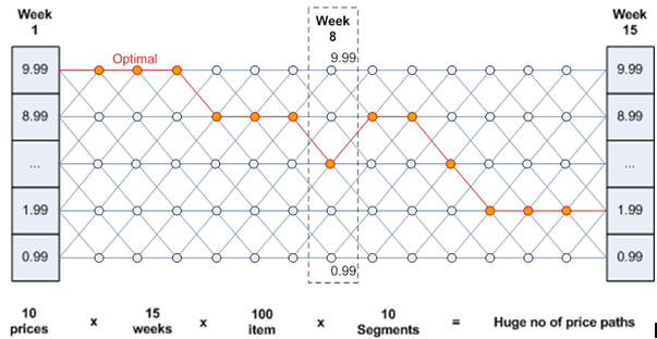
The algorithm uses sophisticated mathematical modeling techniques to analyze all possible solutions to generate the best possible solution. The optimization algorithm is provided an objective (for example, maximize total revenue over all items in the season), business rules or restrictions, and the demand parameters for a particular item. The algorithm analyzes the trade-offs between all possible solutions (see Figure 18-5) and picks the solution that provides the best value for the objective. All the restrictions imposed by the user are treated as required; that is, all possible solutions must satisfy that particular criterion. The only constraint that can be enforced as soft is the sell-through target constraint. The user can make this constraint soft, which tells the optimization that this constraint does not have to be met. Optimization will try to satisfy this constraint, and, if it cannot, it will not return an infeasible or no solution.

Figure 18-5 Optimization Algorithm

To provide a sense of the complexity of the optimization, here is a sample of the trade-offs that are analyzed.

• Is it better to provide a promotion early in the life or wait until later in life to mark down? Will conducting in a promotion now help me given a shallower markdown at a later point in life?

• There are planned promotions scheduled at different points in time. Can these promotions be used and figure out whether an item needs further promotions or markdowns?

• Is providing a promotion at a particular week useful? Will it help meet the sell-through target? Will it increase revenue?

• There are customer segments with different response to price cuts. How can targeted offer provide a promotion that will entice the customer in customer segment A?

• Does providing a promotion or markdown or targeted offer for an item cause a conflict with the imposed business rules? For example, a user might determine that the item cannot be given more than 30% discount.

Offer Optimization Forecasting

Forecasting is applied in the optimization using the demand parameters supplied. Suppose the user wants to generate weekly price recommendations. Depending on the day of the week when markdown is effective, forecasting is adjusted using daily weights to reflect that there are two prices in effect for that week. The same logic applies for promotions as well.

Objective Function

The objective function specified by the user plays a major role in determining which solutions are considered best. For example, if the user specifies the objective function as maximize profit margin, then the algorithm will look for solutions that are superior on profit margin and not necessarily on the other KPIs such as revenue and sales volume. Sometimes, understanding why an item got such a price recommendation might be as trivial as looking at the objective function contribution of that particular item to the objective function.

Constraints

If the objective function focuses on the best possible solution, then constraints work in the opposite direction, by restricting the set of possible solutions. For example, if the objective function says to select the most profitable discount for an item A, a constraint on item A may say it is not possible to have more than certain discount percentage.

Optimization enforces all constraints as required; that is, it finds all the solutions that satisfy all the constraints that are specified by the user. Sometimes, inadvertently, the user might specify conflicting constraints that can result in no solution or unexpected solutions. Often, a resolution can be found by just understanding the implications of individual constraints. More often than not, the user must analyze the interplay between two or more constraints to understand the solution. PRO_RUN_SANITY_CHECK_RSE_VW contains information on the errors/alerts/warnings generated.

OO supports a variety of constraints, and it is essential for the user to understand the purpose and role of each constraint in the optimization.

Frequently Asked Questions

Here are some answers to typical questions that you may encounter.

Question

In a price-zone, there are stores of different inventory levels. Some stores have very high-inventory levels whereas others have low inventory levels. Does OO recommend different recommendations for the zone and such stores separately?

Answer

This is not possible in the current release. You can configure the OO to run either at the price-zone level or at the store-level. If the price-zone level is selected, then all the stores within that price-zone will get the same price recommendations. If you want to have store-level recommendations then you must configure the run-level to be at the store-level and let the algorithm dictate the recommendations. It might be possible if the stores share very similar customer behavior, then they will get similar recommendations.

Question

I am not interested in the promotions; can the product handle only markdowns?

Answer

Yes, the product can handle only markdowns. You can define all the period types as clearance and no period should be defined as regular.

Question

I have a planned promotion and I know when the promotion should occur but I do not know the items and the depth. Can the product recommend items and the depth?

Answer

No, the product requires planned promotion to specify the items, depth, and when. However, if the retailer wants the product to recommend items and depth, then you can specify the promotion and markdown calendar using the interface provided and specify when the promotions and markdowns can be given. Offer Optimization will determine which items should be promoted or the markdown among the set of periods provided. Note that you can specify using the relative calendar option through the UI as well.

Question

Should I use Absolute Calendar or Relative Calendar?

Answer

The two calendars are provided for flexibility in handling two use cases. When all the items are introduced almost at the same time and exit almost at the same time, then it makes sense to use absolute calendar. You can also use the relative calendar in such a use case. When the items are introduced at periodic intervals (for example, summer merchandise is introduced in May, June, and July) then it makes sense to use relative calendar. For example, the absolute calendar in such a scenario would probably say May, June as Regular and July as Clearance. This means that items that were introduced in July are straight away going into a Clearance season. However, the relative calendar begins after the item is introduced. It is defined as the percentage of regular season and the percentage of the markdown season based on the total length of the season available for the item.

Question

Is the Style, Color needed as part of Merchandise Hierarchy?

Answer

Since the product supports fashion apparel, it is expected that the style and color be provided as part of merchandise hierarchy. If the retailer carries non-apparel, then the retailer can specify some generic value for style and color, such as not applicable.

Question

How does Offer Optimization handle the online channel?

Answer

The retailer can specify the online channel as a separate price zone. This means that the price recommendations for brick-and-mortar stores and online-stores will be different. If the retailer does not wish to have different price recommendations, then it is suggested that you combine the online channel into a brick-and-mortar stores.

Question

Can Offer Optimization handle complex promotions?

Answer

Offer Optimization handles only simple promotions (for example, percentage off). It does not handle complex promotions like BOGO.

Question

Can Offer Optimization come up with bundles for complex promotions? How can this be handled?

Answer

Offer Optimization cannot come up with bundles for a promotion. A bundle can be specified using Product Groups under Business Rules. There are three types of product groups supported: Cannot Promote, Must Promote, and Same Pricing in this release.

Question

Is budget constraint over the effective week or over the entire life of the item?

Answer

Remaining budget is assumed to be for the entire remaining life of the item. Budget is used for both promotions and markdowns together; however, you can disregard the budget restriction for promotions or markdowns by turning off the respective flags in RSE CONFIG.

Question

What happens when a user accepts or rejects a recommendation? Do the numbers change for that week? Does it optimize the entire life again?

Answer

In the current release, the metrics in all the Results and Analysis do not reflect the accept, reject, or override price recommendations.

Question

Can Offer Optimization handle any type of price-zone?

Answer

In the current release, Offer Optimization can only take in price-zones that are defined as part of Location Hierarchy.

Question

How does Offer Optimization handle multi-currency support?

Answer

Offer Optimization takes in the historical sales data in the local currency provided. Further, the location in the application can be specified a country locale. Each application run has a location, which is used to tie the price and price-related metrics (for example, revenue) to the specified currency. However, if you want to configure the run to be at level that spans multiple currencies, then you must specify one currency.

Question

How does Offer Optimization support dynamic clustering?

Answer

Any time you change the price-zone or re-cluster the customer segments, it must be re-loaded as part of new hierarchies to Offer Optimization. It is considered a major change to the application as it affects the core data elements. The application will be re-calculating the demand parameters and other relevant optimization inputs based on the new hierarchies. Further, the UI does not offer support to re-group stores within a price-zone based on certain attributes, for example, group stores by sell-through.

Question

How are product images loaded?

Answer

Product images can be loaded via the interface provided. Offer Optimization expects that the images are loaded on an image server (which can be a local server). There is an URL provided (with the image name) that can be accessed by the application. The application searches for the image and populates the UI with the relevant image for that item in the Targeted Offer screen.

Question

What is the difference between Featured Targeted Offers and All Targeted Offers?

Answer

See Figure 18-6 and Figure 18-7. The first is what customer actually sees in the targeted email. It shows four laptops with prices and associated mechanics. In the second figure, when the user visits the online store, the user can see many products that are on promotion and not just the four. Offer Optimization adopts a similar approach in the TO UI components. Featured Targeted Offers are intended to drive the customer to visit the online channel (or store) by showing products, promotions, mechanics that are highly relevant or appropriate for the customer. Once the customer arrives at the online website or store, the customer can see much more deals on the products or All Targeted Offers than just the ones shown in the email.

Figure 18-6 Featured Targeted Offers

Figure 18-7 All Targeted Offers