ofs_aif package

Subpackages

• ofs_aif.batch package
  • Submodules
  • ofs_aif.batch.ml4aml module
  • Module contents
• ofs_aif.dm package
  • Submodules
  • ofs_aif.dm.dm module
  • Module contents
• ofs_aif.graph package
  • Submodules
  • ofs_aif.graph.deepwalk module
  • Module contents
• ofs_aif.ofs_asc package
  • Submodules
  • ofs_aif.ofs_asc.asc module
  • Module contents
• ofs_aif.sanctions package
  • Submodules
  • ofs_aif.sanctions.birth_year_similarity module
  • ofs_aif.sanctions.edq module
  • ofs_aif.sanctions.event_scoring module
  • ofs_aif.sanctions.string_similarity module
  • ofs_aif.sanctions.transformation module
  • Module contents
• ofs_aif.scenario package
  • Submodules
  • ofs_aif.scenario.human_trafficking module
  • ofs_aif.scenario.scenario module
  • ofs_aif.scenario.shell_scenario module
  • Module contents

Submodules

ofs_aif.aif module

This module implements user interface API’s for all the possible ML operations possible.

class aif(connect_with_default_workspace=True)

Bases: object

class AIF: This class implements user interface API’s for ML.

add_model_groups(meta_data_df)

Create segmentation ( model group) using any combination of the meta data available.

Parameters

meta_data_df – Model group creation meta data as pandas data frame

Input data frame parameter description :

• MODEL_GROUP_NAME : Admin defined unique name for the model group. Only alphanumeric character set including underscore, hyphen and space are allowed

• ENTITY_NAME : Logical Entity Name as displayed in metadata section

• ATTRIBUTE_NAME : Logical Attribute Name as displayed in metadata section

• ATTRIBUTE_VALUE : Logical Attribute Value as displayed in metadata section

• LABEL_FILTER : Filter to Identify Entities and Label’s from the table AIF_INVESTIGATED_ENTITY

• FEATURE_TYPE_FILTER : Filters to Identify Feature for the analysis. Options include CASH, WIRE, MI, BOT

Any combination of above type as comma (,) seperated like CASH,MI or MI,CASH,WIRE etc.. is also allowed. Table AIF_VERTICAL_FILTER_LOOKUP is used as look up table for Feature sets to Feature Type

Note:

FEATURE_TYPE_FILTER helps reducing the memory requirement at the model group level. hence optimizes the storage by choosing only required features

Returns

successful message on successfully creating the model groups in AIF system.

Examples:

>>> input_pdf = pd.DataFrame({'MODEL_GROUP_NAME'   : ["LOB1","LOB1"],
>>>                         'ENTITY_NAME'         : ["Customer","Customer"],
>>>                         'ATTRIBUTE_NAME'      : ["Business Domain(s)","Jurisdiction Code"],
>>>                         'ATTRIBUTE_VALUE'     : ["General","Americas"],
>>>                         'LABEL_FILTER'        : ["CUST","CUST"],
>>>                         'FEATURE_TYPE_FILTER' : ["WIRE_TRXN/MI_TRNX/CASH_TRNX/BACK_OFFICE_TRXN","WIRE_TRXN/MI_TRNX/CASH_TRNX/BACK_OFFICE_TRXN"]
>>>                         })
>>>
>>> aif.add_model_groups( input_pdf )

add_new_attribute_values_for_model_group_metadata(df, remove=False)

Add new attributes to the AIF system, so that they can be used as metadata for creating model groups.

Parameters

• entity_attribute_value_df – Input Data frame with ENTITY & ATTRIBUTES & VALUES column should be provided ( Refer example below )

• remove – Options TRUE/FALSE. If TRUE, Attribute values will be removed under metadata for model group creation. Else new value will be added

Returns

Successful message on successfully adding/removing the attribute values. Returns error message if fails…

Example:

>>> pdf = pd.DataFrame({'ENTITY' : ["Account"],
>>>                    'ATTRIBUTE_NAME' : ["Jurisdiction Code"],
>>>                    'ATTRIBUTE_VALUE' : ["Channai"],
>>>                    'ATTRIBUTE_CODE' : ["MDRS"]
>>>                   })
>>>
>>> aif.add_new_attribute_values_for_model_group_metadata(pdf, remove = False)

add_to_modeling_dataset(pandas_df_list=None, key_var='ENTITY_ID', label_var='SAR_FLG', overwrite=True, reset=False, osot=False, amles=False)

Merge all input data frames and create modeling dataset.

Parameters

• pandas_df_list – list of transformed data frames.

• key_var – key variable to be used for merging the results. all input data frames is expected to contain key column, else merge wil fail.

• label_var – Name of the Target/Label variable if present in the input/resultant data frame .

• overwrite – Boolean flag with Options as True/False. If True, keeps overwriting existing column from the new resultant frame. Else will leave as it is.

• reset – Boolean flag with Options as True/False. If True, resets modeling data to None.

• osot – Boolean flag with Options as True/False. True for osot data and False for osit data.

Note:

overwrite flag overwrites only those columns of modeling data, which are part of current API call. Columns not part of the current API call will not be overwritten. reset flag deletes all the modeling data prior to current API call.

Returns

True/False. True on succesful operation. On successful operation, modeling data is created and saved inside the class object.

Example:

>>> aif.add_to_modeling_dataset( [ ts_pdf, jbm_pdf, graph_embeddings_pdf, average_deposit_pdf, NB_PDF ], overwrite = True )

auc_summary(osot=False)

Extracts the results of a given aif run. The returned results will contain the model, model_gid, algo and AUC performance of the top_N models for each by_type in the run. The columns: Model denotes the unqiue ID of a model, Model_gid differentiates models using same algorithm but assigned with different run paramters within clsf_grid, Algo denotes the shortnames of ML algorithms used for model build - in this case if for e.g., the run contained xgboost model type with several possible hyperparamter combinations, only one xgboost model will be returned.

Param

None

Returns

AUC summary dataframe

Example:

>>> aif.auc_summary()

auc_summary_detailed()

Similar to auc_summary() with by_type=”All” option

Param

None

Returns

AUC summary dataframe

Example:

>>> aif.auc_summary_detailed()

close_ecm_connection()

Closes the existing open ECM connection.

Returns

None

Examples 1:

>>> aif.close_ecm_connection().

close_open_plots()

classes all open plots in the current python session.

Param

None

Returns

None

Example:

>>> aif.close_open_plots()

configure_investigation_guidance(model_group_name=None, model_group_scenario_name=None, feature_list=[], top_n=10, rule_type='any', guidance_text=None, overwrite=False)

Store the top N features list with guidance text in AIF_INVESTIGATION_GUIDANCE table. User is allowed to set guidance text for set of features either at local or global level.

• local : limited to particular model group only. model group should not be None in this case

• global: avilable at global level if model group name and scenario is not defined.

Parameters

• model_group_name – Model group name

• model_group_scenario_name – Model group scenario

• feature_list – List of features list to store

• top_n – Number of top contributing features to search for feature_list

• rule_type – all or any features to be in the feature’s list. Default to ‘any’ - all : all configured features to be in top N - any : any of the congigured features to be in top N

• guidance_text – Guidance text correspondence to features_list provided.

• overwrite – Boolean True/False. If True, overwrite the existing entry in DB

Returns

Successful message or error messages if any…

Examples:

>>> #features list to search in top 5 contributing features
>>> aif.configure_investigation_guidance(model_group_name='LOB1', feature_list=['f1','f2'], top_n=5, guidance_text='Possibly a Human Trafficking')
>>>
>>> #features list to search in top 10 contributing features
>>> aif.configure_investigation_guidance(model_group_name='LOB1', feature_list=['f1','f2','f3','f4','f5'], top_n=10, guidance_text='fraud')

create_definition(model_group_name=None, model_group_scenario_name=None, save_with_new_version=False, cleanup_results=False, version=None)

API creates unique definition using Model Group and Model Group Scenario ( optional ) for a given Notebook.

Parameters

• model_group_scenario_name – Name of the Model Group , as per it created in AIF-Admin notebook.

• save_with_new_version – Boolean flag with options True/False. It helps creating history of models/outputs for a given definition. Any version can be chosen at later point in time.

• cleanup_results – Boolean flag with options True/False. When set to True, deletes all the outputs due to previous executions.

• version – when multiple versions of the definitions are created, version is supplied to pick the required version of the definition. Default value is None means MAX version of the definition.

Returns

Return successful message on completion, and proper error message on failure.

Examples:

>>> aif.create_definition( model_group_name = "CORPORATE AND INSTITUTIONAL" ,
>>>                        model_group_scenario_name = "SHELL",
>>>                        save_with_new_version = False,
>>>                        cleanup_results = False,
>>>                        version = None )
Definition creation successful...
True

create_instance(connect_with_default_workspace=True)

Creating instance of the class aif. Object of this class is used as reference/handle to drive all the other UI API’s implemented.

Parameters

connect_with_default_workspace – Boolean True/False. True if to connect with default compliance studio workspace.

Returns

None

Example:

>>> aif.create_instance()

deploy(technique=None)

To deploy the selected Model. This API creates an entry in the OFS_AUTO_ML_DEPLOYED_MODEL for the Model deployed against the V_DEFINITION_ID.

Parameters

technique – The model to be deployed.

Returns

None

Examples:

>>> aif.deploy(technique = 'XGB1')

drop_features_from_modeling_dataset(feature_list=None)

The API drops the specified features/columns from the modeling data.

Parameters

feature_list – list of features to be dropped from modeling dataset as python list.

Returns

None Modeling data gets updated internally. use self.get_modeling_dataset to get the updated modeling data into python session.

Example:

>>> aif.drop_features_from_modeling_dataset( feature_list = ['Feature1', 'Feature2'] )

eda_auto_sample_proportion(input_pdf=None, label_var='SAR_FLG', use_labels=True)

To compute Sampling proportion based on the distribution of labels in the dataset.

• 0.33 -> If Num of Bads < 100

• 0.5 -> If Num of Bads < 150

• 0.66 -> If Num of Bads < 200

• 0.75 -> If Num of Bads < (250 + 50*0.2)

• 0.8 -> Otherwise

Note:

Bads refers to the records where the label is set to 1 or in this case where SAR_FLG is enabled.

Parameters

• input_pdf – The dataframe for which the the Sampling proportion has to be computed.

• label_var – Target Variable

• use_labels – Boolean flag to indicate if data is supervised or unsupervised. Defaults to True.

Returns

Training proportion

eda_bivariate_analysis_plot(input_pdf=None, feature_include=None, feature_exclude=None, label_var='SAR_FLG', use_labels=True)

This API helps in determining the relationship between two variables. It comes under Bi-variate Analysis in EDA. Exploratory data analysis(EDA) is an approach which involves analyzing the data sets to summarize their main characteristics, using statistical graphics and other data visualization methods. If more than 2 features are passed, it provides plot for all possible combinations of variables.

Parameters

• input_pdf – Input data set

• feature_include – List of features to be included.

• feature_exclude – List of features to be excluded.

• label_var – Target Variable Default set to SAR_FLG

Returns

Bi-variate Analysis Plot.

Examples:

>>> aif.eda_bivariate_analysis_plot( input_pdf = modeling_EDA_pdf)

eda_categorical_summary(input_pdf=None, feature_include=None, feature_exclude=None, key_var='ENTITY_ID', use_labels=True)

This API provides Categorical Summary under Exploratory Data Analysis (EDA) on the Input dataset which is the Stage 2 transformed Dataset. Exploratory data analysis is an approach which involves analyzing the data sets to summarize their main characteristics, using statistical graphics and other data visualization methods. This technique is applicable on Categorical features only.

Parameters

• input_pdf – Input dataset

• feature_include – List of features to be included.

• feature_exclude – List of features to be excluded.

• key_var – Key Variable (Entity id in this case) Default set to ENTITY_ID.

Returns

Categorical Summary.

Examples:

>>> aif.eda_categorical_summary( input_pdf=modeling_EDA_pdf,
>>>             feature_exclude=['TOT_DEPST_AM_MEDIAN'])
>>> aif.eda_categorical_summary( input_pdf=modeling_EDA_pdf,
>>>             feature_include=['TOT_DEPST_AM_CLIP','TOT_DEPST_CT_CLIP'])
>>> aif.eda_categorical_summary( input_pdf = modeling_EDA_pdf )
Display dataframe with below information:
    - Variable
    - Unique values
    - Unique value count
    - Missing count
    - Missing percentage

eda_correlation_heat_map_plot(input_pdf=None, feature_include=None, feature_exclude=None, label_var='SAR_FLG', use_labels=True)

This API provides the Correlation Heatmap for Numerical Variables under Exploratory Data Analysis (EDA) on the Input dataset which is the Stage 2 transformed Dataset. Exploratory data analysis is an approach which involves analyzing the data sets to summarize their main characteristics, using statistical graphics and other data visualization methods. This technique is applicable on Numerical features only. Analysis of `Correlation Heatmap helps in removing the multi-collinearity to some extent.

Parameters

• input_pdf – Input dataset

• feature_include – List of features to be included.

• feature_exclude – List of features to be excluded.

• label_var – Target Variable Default set to SAR_FLG

Returns

Correlation Heat map

Examples:

>>> aif.eda_correlation_heat_map_plot( input_pdf = modeling_EDA_pdf )

eda_frequency_distribution_plot(input_pdf=None, feature_include=None, feature_exclude=None, label_var='SAR_FLG', key_var='ENTITY_ID', use_labels=True)

This API provides the Frequency Distribution Plot of Categorical Variables under Exploratory Data Analysis (EDA) on the Input dataset which is the Stage 2 transformed Dataset. Exploratory data analysis is an approach which involves analyzing the data sets to summarize their main characteristics, using statistical graphics and other data visualization methods. This technique is applicable on Categorical features only.

Parameters

• input_pdf – Input dataset

• feature_include – List of features to be included.

• feature_exclude – List of features to be excluded.

• label_var – Target Variable Default set to SAR_FLG

• key_var – Key Variable (Entity id in this case) Default set to ENTITY_ID.

Returns

Frequency Distribution Plot for each of the variable.

Examples:

..code-block:: python

>>> aif.eda_frequency_distribution_plot( input_pdf = modeling_EDA_pdf,
    feature_include=['TOT_DEPST_AM_CLIP','TOT_DEPST_CT_JMP_P100',
                    'TOT_DEPST_AM_TREND','TOT_DEPST_AM_JMP_P100'] )

eda_information_value(input_pdf=None, feature_include=None, feature_exclude=None, label_var='SAR_FLG')

This API gives the Information Value of each of the variable. It comes under Uni-variate Analysis in EDA.

• Information Value (IV) -> A numerical value that quantifies the predictive power of an independent continuous variable x in capturing the binary dependent variable y. In case of categorical variables, they are transformed to bins and then the IV is computed for them.

• Exploratory data analysis(EDA) -> EDA is an approach which involves analyzing the data sets to summarize their main characteristics, using statistical graphics and other data visualization methods.

Parameters

• input_pdf – Input data set

• feature_include – List of features to be included.

• feature_exclude – List of features to be excluded.

• label_var – Target Variable Default set to SAR_FLG

Returns

Information Value of each of the variable.

Examples:

>>> aif.eda_information_value( input_pdf = modeling_EDA_pdf)
>>>
>>> aif.eda_information_value( input_pdf = Stage_2_data,
>>>             feature_exclude=['TOT_DEPST_CT_MEAN','TOT_DEPST_CT_TREND','TOT_DEPST_CT_MEDIAN'])
Display dataframe with below information:
    - woe_variable
    - total_iv

eda_numerical_summary(input_pdf=None, plot=True, feature_include=None, feature_exclude=None, key_var='ENTITY_ID', label_var='SAR_FLG', use_labels=True)

This API provides Numerical Summary under Exploratory Data Analysis (EDA) on the Input dataset which is the Stage 2 transformed Dataset. Exploratory data analysis is an approach which involves analyzing the data sets to summarize their main characteristics, using statistical graphics and other data visualization methods. This technique is applicable on Numerical features only.

Parameters

• input_pdf – Input dataset

• plot – Boolean (True/False) If set to True, the Density plot will also be plotted. If set to False, only the Numerical Summary will be displayed. Default set to True.

• feature_include – List of features to be included.

• feature_exclude – List of features to be excluded.

• key_var – Key Variable (Entity id in this case). Default set to ENTITY_ID.

• label_var – Target Variable (‘SAR_FLG’)

Returns

Numerical Summary and/or the Density plot.

Examples:

>>> aif.eda_numerical_summary( input_pdf = modeling_EDA_pdf, plot = True,
>>>                 feature_exclude = ['SAR_FLG'] )

>>> aif.eda_numerical_summary( input_pdf=modeling_EDA_pdf, plot = False,
>>>                 feature_exclude = ['SAR_FLG'] ))
Display dataframe with below information:
    - Variable
    - Min
    - Max
    - Missing count
    - Missing percentage
    - Mean
    - Q1
    - Median
    - Q3
    - Skewness
    - Kurtosis

eda_sampling(input_pdf=None, label_var='SAR_FLG', eda_sample_proportion=None, use_labels=True)

To perform Exploratory Data Analysis on a sampled rather than the entire dataset. Stratified Sampling based on the percentage (eda_sample_proportion) provided in the input. This API returns a sampled dataset for EDA. If the Sample proportion is not provided, it will be calculated based on the following formula:

• 0.33 -> If Num of Bads < 100

• 0.5 -> If Num of Bads < 150

• 0.66 -> If Num of Bads < 200

• 0.75 -> If Num of Bads < (250 + (total bad)*0.2)

• 0.8 -> Otherwise

Parameters

• input_pdf – The input dataset which has to be sampled.

• label_var – Target Variable

• eda_sample_proportion – Sample proportion which should be used to perform Sampling.

Returns

Sampled dataset

Examples:

>>> aif.eda_sampling( input_pdf = modeling_pdf, eda_sample_proportion = None )
Auto data partition applied.
SAR count in input data : 619
EDA sample proportion   : 0.8

eda_sar_distribution(eda_data_pdf=None, label_var='SAR_FLG')

This API gives the details of SAR distribution in the data.

Parameters

• eda_data_pdf – Input data which contains the label(target variable) as well.

• label_var – Target variable

Returns

Count of individual values in the label.

Examples:

>>> aif.eda_sar_distribution( modeling_EDA_pdf )
SAR_FLG
0    211
1     68
Name: SAR_FLG, dtype: int64

eda_time_series_plot(x=None, feature_include=None, feature_exclude=None, plot_type='line')

Time series EDA on AIF behavioral data

Parameters

• x – AIF behavioral time series data as pandas data frame

• feature_include – Filters to select features from input data frame.

• feature_include – Filters to remove features from input data frame.

• plot_type – options line or box

Returns

Display time series EDA plots.

Example:

>>> aif.set_plot_dimension( width = 14, height = 8 )
>>> aif.eda_time_series_plot( x = B_OSIT_PDF , feature_include = ['TOT_DEPST_AM', 'TOT_DEPST_CT'], plot_type = "line" )
>>> aif.show_plots()

>>> aif.set_plot_dimension( width = 14, height = 8 )
>>> aif.eda_time_series_plot( x = B_OSIT_PDF , feature_include = ['TOT_DEPST_AM', 'TOT_DEPST_CT'], plot_type = "box" )
>>> aif.show_plots()

enable_attributes_as_model_group_metadata(df, disable=False)

Enable/Disable attributes as metadata for model group creations.

Parameters

• entity_attribute_df – Input data frame formed with respect to showUnusedAttributesInModelGroupMetadata().

• disable – Options TRUE/FALSE If TRUE : Attributes will be disabled under metadata for model group creation. By default its FALSE ( means enable attribute )

Returns

Successful message on successfully enabling/disabling the attributes. Returns error message if fails…

Example:

>>> pdf = pd.DataFrame({'ENTITY' : ["Customer"],  'ATTRIBUTES' : ["Occupation"] })
>>>
>>> aif.enable_attributes_as_model_group_metadata(pdf , disable = False )
>>> OR
>>> aif.enable_attributes_as_model_group_metadata(pdf , disable = True )

feature_contribution_plot(model_id=None, at_qprobs=[0.05, 0.5, 0.99], plot=True, entity_id=None, key_var='ENTITY_ID', n_top_contrib=None)

Display Feature Contribution (Local Explanation method) plots

Parameters

• model_id – model id to be passed from list of models stored during training.

• entity_id – entity for which explainability is required

• n_top_contrib – Number of top contributing features to display on Y-axis in feature contribution plot

• at_qprobs – Quantiles for Feature Contribution.

• plot – Display plots or not. Boolean True/False. Default is True

• key_var – key variable in dataset

Returns

feature contributions

Examples:

>>> import aif
>>> ## SELECT OBSERVATION WITH PARAMETER at_qprobs
>>> aif.feature_contribution_plot(model_id='XGB1',
>>>                                key_var='ENTITY_ID',
>>>                                at_qprobs={'age':[18,19]},
>>>                                n_top_contrib=10)
>>>
>>> ## SPECIFIED QUANTILES WITH PARAMETER at_qprobs
>>> aif.feature_contribution_plot(model_id='XGB1',
>>>                                key_var='ENTITY_ID',
>>>                                at_qprobs=[0.1,0.3,0.6,0.9],
>>>                                n_top_contrib=10)
>>>
>>> ## SPECIFIED ALL WITH PARAMETER at_qprobs
>>> aif.feature_contribution_plot(model_id='XGB1',
>>>                                key_var='ENTITY_ID',
>>>                                at_qprobs='all',
>>>                                n_top_contrib=10)

>>> aif.feature_contribution_plot( model_id = 'XGB1', plot = True )

>>> aif.feature_contribution_plot( model_id = 'XGB1', plot = True )
Display dataframe with feature contribution information:
    - Key_Column
    - Row_index
    - Key_Value
    - _BASE_
    - TOT_DEPST_AM_CLIP
    - TOT_DEPST_CT_MEAN
    - TOT_DEPST_CT_JMP_P100
    - TOT_DEPST_AM_JMP_P75
    - TOT_DEPST_CT_JMP_P75
    - TOT_DEPST_AM_MEDIAN
    - BENFORD_DEVIATION

feature_importance_plot(model_id=None, label_var='SAR_FLG', scaling=False)

Display Permuted Feature Importance(Global Explanation method) plots for input features

Parameters

• model_id – model id to be passed from list of models stored during training.

• label_var – response variable. Default is ‘SAR_FLAG’

• scaling – Boolean indicating whether user wants scaled values.

Returns

plots

Examples:

>>> import aif
>>> aif.feature_importance_plot( model_id = 'XGB1', scaling=True )

>>> import aif
>>> aif.feature_importance_plot( model_id = 'XGB1', scaling=False )

get_behavioral_data(osot=False)

Get time series data as pandas data frame.

Parameters

osot – Boolean flag to indicate data set type ( OSIT or OSOT ). False: (default) For OSIT data set. ( Model build dataset ) True: For OSOT dat aset.

Returns

Behavioural data as pandas data frame.

Example:

>>> B_OSIT_PDF  = aif.get_behavioral_data();
>>> OR
>>> B_OSIT_PDF  = aif.get_behavioral_data(osot = True);

get_cx_connection()

get_data_source_connection(data_source=None)

get_dynamic_jmp_desc(feature, thres, value)

get_ecm_connection()

return the ECM connection object.

Returns

cx_Oracle connection object.

Examples 1:

>>> aif.get_ecm_connection().

get_golden_data()

Simulated test data part of the application. Insert Golden Data into Oracle Table This is just one time activity. Data is available under $FIC_HOME/AIF_Golden_Data folder ( BD Home Directory ). Execute insert scripts available under AIF_Golden_Data. Connect to a RDBMS schema configured for AIF and run/execute all sql files.

Param

None

Returns

True on success. Sets the behavioral & Non-Behavioral data within class members.

Example:

>>> aif.get_golden_data()

get_investigation_guidance(model_group_name=None, model_group_scenario_name=None, feature_list=[], feature_contrib_dict=None)

This API retrieves the features set with guidance text from table AIF_INVESTIGATION_GUIDANCE while scoring process, and Investigation summary also gets prpeared which is mainly used for iHub.

If model group is None, then this API assumes guidance for features are set at global level. Firstly, API will look for the guidance at local level (model group is not None) and if not found then it searches at global level. Guidance at local model level will always take priority if it was set at both local as well as global level.

Parameters

• model_group_name – Model group name

• model_group_scenario_name – Model group scenario

• feature_list – [optional] List of top features in terms of its contribution. If None, guidance text for all top N features will be retrieved.

• feature_contrib_dict – This is feature’s contrib dcitionary that will be passed internally during scoring process. Mandatory only for creating investigation summary because it contains probability scores from the scoring batch. It is mailny for showing information in iHub.

Returns

It returns 2 dataframs: - dataframe showing Guided text for corresponding top N features - dataframe showing Investigation summary

Examples:

>>> #All top N features
>>> aif.get_investigation_guidance(model_group_name='LOB1', model_group_scenario_name = 'Shell')
>>>
>>> #passed feature's contribution list
>>> a, b = aif.get_investigation_guidance(model_group_name='LOB1', feature_list=['f1','f2','f3','f4','f5'])

get_model_features(mdl_id=None)

Gets final model features of the specified model

get_model_group_id(name='')

API returns the model group ID for a given model group name. Every model group name will have unique model group ID in AIF system.

Parameters

name – Input model group name as python string.

Returns

Model group ID as python string

Examples:

>>> aif.get_model_group_id('LOB1')

get_model_group_name()

API returns the model group name on which current ML definition is created.

Returns

Model group name as python string

Examples:

>>> aif.get_model_group_name('Notebook_ID_1')

get_model_group_scenario_id(name=None)

API returns the model group scenarion ID for a given model group scenario name. Every model group scenario name will have unique model group scenario ID in AIF system.

Parameters

name – Input model group scenario name as python string.

Returns

Model group scenario ID as python string

Examples:

>>> aif.get_model_group_scenario_id('Cash')

get_model_group_scenario_name()

API returns the model group scenario name on which current ML definition is created.

Returns

Model group scenario name as python string. Returns None if definition does not contain model group scenario.

Examples:

>>> aif.get_model_group_scenario_name()

get_modeling_dataset(osot=False)

Get modeling data in current session

Param

None

Returns

modeling data as pandas data frame.

Example:

>>> Stage_2_OSIT_pdf = aif.get_modeling_dataset()

get_non_behavioral_data()

Get non behavioral data as pandas data frame.

Param

None

Returns

Non Behavioural data as pandas data frame.

Example:

>>> NB_PDF = aif.get_non_behavioral_data();

get_notebook_id()

This is an internal API. Not recommended for general usage. Returns notebook ID(Unique User Reference ID ) for a given class instance.

Returns

Notebook ID as string

Examples:

>>> aif.set_notebook_id('Notebook_ID_1')

get_osot_auc(x_osot=None, y_osot=None, label_var='SAR_FLG', model_list=None)

load auc summary for OSOT data

Parameters

• x_osot – [Optional] (Pandas-Dataframe) OSOT input dataframe

• y_osot – [Optional] (Pandas-Dataframe) OSOT target dataframe

• label_var – [Optional] target variable. Default is ‘SAR_FLG’

Model_list

[Optional] (List, str, None) List of model-ids for which OSOT AUCs to be computed. If None, AUCs for all stored models will be shown Valid Options are:

• model_list = ‘XGB1’, display Output for single model

• model_list = [‘XGB1’,’ADB1’], display output for multiple models

• model_list = None, display for all stored models during the fit

Returns

auc dataframe for osot

Note:

OSOT data will be retrieved from DB tracking table if it was supplied during the fitting of model. Provided Validation_type=’BOTH’ in trainer_params

Example:

>>> aif.get_osot_auc()
Model       Validation
ADB1        0.737648
WOELR1      0.745880
GB1         0.754614

get_osot_perf_metrics(x_osot=None, y_osot=None, performance_metric='auc_change', label_var='SAR_FLG', model_list=None)

Compute OSOT performance metrics which includes AUC change% and Population Stabiliy Index values

Parameters

• x_osot – [Optional Parameter] (Pandas-Dataframe) OSOT input dataframe

• y_osot – [Optional Parameter] (Pandas-Series) OSOT target data

• performance_metric –

  Performance metric for OSOT data. Default is ‘auc_change’ Valid options are:

  • auc_change

  • decile_psi

  • total_psi

• label_var – [Optional].Target variable. Default is ‘SAR_FLG’

• model_list –

  [Optional] (List, str, None) List of model-ids for which performance metrics to be computed. Defaults to None. If None, Performance metrics will be shown for the Best model Valid Options are:

  • model_list = None, If None, display output for best model by auc.

  • model_list = ‘All’, display output for all models

  • model_list = ‘XGB1’, display Output for single model

  • model_list = [‘XGB1’,’ADB1’], display output for multiple models

Returns

AUC %change and Population Stability index dataframes

Note:

OSOT data will be retrieved from DB tracking table if it was supplied during the fitting of model. Provided Validation_type=’BOTH’ in trainer_params

Examples:

>>> aif.get_osot_perf_metrics(model_list=['XGB1','ADB1'])
model  train_auc  osot_auc  pct_change
0  XGB1   0.765562  0.765562         0.0
1  ADB1   0.807004  0.807004         0.0

>>> aif.get_osot_perf_metrics(performance_metric='total_psi')
Model   Total PSI
0  ADB1  186.503956

>>> aif.get_osot_perf_metrics(performance_metric='total_psi', model_list=['XGB1','ADB1'])
Model   Total PSI
0  XGB1   90.730313
1  ADB1  186.503956

get_osot_perf_plots(x_osot=None, y_osot=None, label_var='SAR_FLG', performance_metric='Confusion Matrix', cutoff_method='Kappa', custom_threshold=None, model_list=None)

Performance plots on the Validation data(during Model Development) and on OSOT data

Parameters

• x_osot – (Pandas-Dataframe): OSOT input dataframe

• y_osot – (Pandas-Series): OSOT target data

• label_var – Target variable. Default is ‘SAR_FLG’

• performance_metric –

  Metric for Visualization. Default is ‘Confusion Matrix’ Valid options are:

  • ROC Curve

  • PR Curve

  • Prediction Density

  • F1 Curve

  • Kappa Curve

  • Confusion Matrix with cutoff_method=’kappa’

  • Confusion Matrix with cutoff_method=’f1’

  • Confusion Matrix with cutoff_method=’ks’

  • Confusion Matrix with custom_threshold

• cutoff_method – F1 or Kappa or Ks in case performance_metric is Confusion Matrix. Param custom_threshold should be None in this case.

• custom_threshold – Threshold value passed by user. Example: custom_threshold=0.7 If not None, it will take precedence over cutoff-method

• model_list – Model for which Visualization is needed

Returns

Performance plots

Note:

OSOT data will be retrieved from DB tracking table if it was supplied during the fitting of model. Provided Validation_type=’BOTH’ in trainer_params

get_production_data_query(osot_end_month=None)

Internal API to get data during scoring/predict. There are dependent API to be called before invoking this API.

Parameters

osot_end_month – Default value is None. This parameter is applicable only during scoring to get latest month data. Not applicable for sandbox.

Returns

temporary prod table with data

Examples:

>>> aif.get_production_data_query(osot_end_month='201802')

get_sql_alchemy_connection()

get_sql_alchemy_engine()

get_workspace()

Get workspace details

initialize_connection()

Initialize workspace connection

is_production()

Internal API to switch between sandbox & production. Not intended for general usage.

load_object(key=None)

Loads the object saved using self.save_object()

Parameters

key – Unique name of the object storage ( same as it used during self.save_object() ).

Returns

valid python object on successful execution.

Example:

>>> data_pdf = aif.load_object( key = 'AIF_DATA')

load_trainer_status()

Used to load the previously saved internal model object.

Param

None

Returns

Internal model object

load_transformation_results(transformation_key=None)

Load transformation is a counter part of save_transformation_results() API. Retrieves results from the storage and makes it available in the current python session.

Parameters

transformation_key – key used while saving the transformation results using save_transformation_results.

Returns

saved results as pandas data frame.

Examples:

>>> #required imports specific to implementation.
>>> from ofs_auto_ml.feature_transform import ts_clustering as ts
>>>
>>> #creating object
>>> ts_obj = ts.TsClustering(bmp_type=['clip','trend'], multiv_max_clus=100, multiv_max_freq=5, max_clus=20 )
>>>
>>> #calling method : fit_transform
>>> ts_pdf = ts_obj.fit_transform( B_OSIT_PDF, key_var="ENTITY_ID",ts_var="MONTH_ID", feature_include = ["TOT_DEPST_AM", "TOT_DEPST_CT"] )
>>>
>>> aif.save_transformation_results({ 'Time Series Clustering' : ts_pdf })
>>>
>>> ts_pdf = self.load_transformation_results('Time Series Clustering')

load_transformations(key=None)

Load transformation objects whenever needed ( mainly during scoring ). load_transformations() loads only those transformations, which are saved using save_transformations()

Parameters

key – Transformation key used while saving using the API self.save_transformations()

Returns

returns transformation object for the specified key.

Example:

>>> from ofs_auto_ml.feature_transform import ts_clustering as ts
>>> ts_obj = self.load_transformations(key = 'Time Series Clustering')

merge(pandas_df_list, key_var='ENITITY_ID', label_var='SAR_FLG', overwrite=True, osot=False, amles=False)

Customized merge used for concatenation multiple dataframes for AIF use case.

Parameters

• pandas_df_list – list of dataframes to merge

• key_var – Identity column. Default “ENTITY_ID”

• label_var – target variable. Default ‘SAR_FLG’

• overwrite – Boolean True/False. Overwrite existing column’s data if True.

• osot – Boolean True/False. If running for out-time data (OSOT), it should be True.

• amles – Boolean True/False. If running for amles use case, it should be True

Returns

resulted dataframe

merge_generic(pandas_df_list, key_var='ENITITY_ID', overwrite=True)

merge multiple dataframes into single

model_performance_plot(performance_metric='F1 Curve', osot=False)

This API helps in evaluating the Performance of the Model using various Visualizations. The current implementation supports following plots:

1. F1 Curve

2. Kappa Curve

3. Prediction Density

4. Precision Recall Curve

5. ROC Curve

Parameters

• performance_metric – The performance metric for which plot is needed. Default set to “F1 Curve”

• osot – Boolean(True/False) If set to True, display performance plots for OSOT data. Make sure validation_type = ‘BOTH’ in trainer_params

Returns

Plot as per the metric selected

Examples:

>>> aif.model_performance_plot(performance_metric = "Prediction Density")

>>> aif.model_performance_plot(performance_metric = "ROC Curve")

>>> aif.model_performance_plot(performance_metric = "Precision Recall Curve")

>>> aif.model_performance_plot(performance_metric = "Kappa Curve")

>>> aif.model_performance_plot(performance_metric = "F1 Curve")

modify_model_groups(meta_data_df)

Modify model group using the combination of input metadata.

Parameters

meta_data_df – Input pandas data frame formed using available metadata.

Input metadata data frame to be passed for modifying model groups should be similar to the one used while adding/creating a model group. Additional columns required for modifying model groups are

1. ACTION_TYPE : ADD/REMOVE If ADD : combination will be added. If REMOVE : Combination will be removed.

2. DISABLE_GROUP : Y/N If Y : Whole model group will be disabled. By default its N.

For Update : Update should be carried out as REMOVE & ADD as 2 step process. REMOVE the combination to be updated & ADD the new combination.

Returns

Successful message on successfully adding model groups. Returns error message during failures…

Example:

>>> modify_pdf = input_pdf = pd.DataFrame({'MODEL_GROUP_NAME'     : ["LOB1"],
>>>                                          'ENTITY_NAME'         : ["Customer"],
>>>                                          'ATTRIBUTE_NAME'      : ["Business Domain(s)"],
>>>                                          'ATTRIBUTE_VALUE'     : ["General"],
>>>                                          'LABEL_FILTER'        : ["CUST"],
>>>                                          'FEATURE_TYPE_FILTER' : ["WIRE_TRXN/MI_TRNX/CASH_TRNX/BACK_OFFICE_TRXN"]
>>>                                          'ACTION_TYPE'         : ["REMOVE"],
>>>                                          'DISABLE_GROUP'       : ["N"]
>>>                                          })
>>>
>>> modify_pdf = pd.DataFrame({'MODEL_GROUP_NAME' : ["LOB1"],
>>>                          'ENTITY_NAME'         : [""],
>>>                          'ATTRIBUTE_NAME'      : [""],
>>>                          'ATTRIBUTE_VALUE'     : [""],
>>>                          'ACTION_TYPE'         : [""],
>>>                          'DISABLE_GROUP'       : ["Y"]
>>>                          })
>>>
>>> aif.modify_model_groups( modify_pdf )

obtain_investigation_details()

Provides additional investigation details in iHUB.

Returns

Investigation details as a dictionary of pandas data frames.

Examples 1:

>>> aif.get_case_information().

partial_dependency_plot(model_id=None, feature_include=None, n_top_features=6, n_bottom_features=2, num_ice_lines=20, label_var='SAR_FLG')

Display Model Response (Mix of Local and Global Explanation) plots

Parameters

• model_id – model id to be passed from list of models stored during training.

• feature_include – Custom features for Model Response

• n_top_features – Number of most important features to be considered for Model Response. Default 6

• n_bottom_features – Number of least important features to be considered for Model Response. Default 2

• num_ice_lines – Number of lines to be drawn in the ICE plot. Default 20

• label_var – response variable. Default is ‘SAR_FLAG’

Returns

plots

Examples:

>>> import aif
>>> aif.partial_dependency_plot(model_id='XGB1',
>>>                            label_var='SAR_FLG',
>>>                            feature_include=['feature 1','feature 2'],
>>>                            n_top_features=10,
>>>                            n_bottom_features=4,
>>>                            num_ice_lines=50)
>>> OR
>>> aif.partial_dependency_plot( model_id = 'XGB1',
                                feature_include = ['TOT_DEPST_AM_MEDIAN'])

refresh_sar(model_group_name=None)

Update SAR_FLG for entities with latest status from investigated entity

save_feature_description(overwrite=False, **kwargs)

Save the details of the User Defined Transformation in the OFS Auto ML tracking table (OFS_AUTO_ML_OUTPUT_TRACKING). This information is stored at Definition-level.

Parameters

• overwrite – Boolean(True/False) indicating whether to overwrite the existing entry in the OFS_AUTO_ML_OUTPUT_TRACKING table under the v_output_name : FEATURE_DESCRIPTION By default, set to False.

• kwargs – Key-word Arguments provided by the User for each of the feature in the following format: [‘FEATURE’,’FEATURE_TAG’,’FEATURE_DESCRIPTION’] or in the form of a data frame.

Examples:

>>> # Store the information for one feature
>>> aif.save_feature_description(overwrite=False, feature1=['ATM_TRXN_IN_AM_MEDIAN', 'Median of ATM Transactions Incoming Amount', 'Median of Amount coming in through ATM Transactions'])
>>> # Overwrite the Existing Entry in DB (if present)
>>> aif.save_feature_description(overwrite=True, feature1=['ATM_TRXN_IN_AM_MEDIAN', 'Median of ATM Transactions Incoming Amount', 'Median of Amount coming in through ATM Transactions'],
>>>                        feature2=['ATM_TRXN_OUT_AM_MEDIAN', 'Median of ATM Transactions Outgoing Amount', 'Median of Amount going out through ATM Transactions'])
>>>
>>> # NOTE:User will be informed if the entry is overwritten.
>>>
>>> # Provide the input in data frame format
>>> print(df1)
FEATURE                             FEATURE_TAG                                 FEATURE_DESCRIPTION
ATM_TRXN_IN_AM_MEDIAN       Median of Incoming ATM Transactions         Median of Amount coming in through ATM Transactions
ATM_TRXN_OUT_AM_MEDIAN      Median of Outgoing ATM Transactions         Median of Amount going out through ATM Transactions
>>> aif.save_feature_description(overwrite=True, feature_df=df1)

save_object(key=None, value=None, description=None)

save python objects permanently. Load them whenever needed.

Parameters

• key – Unique name for the object storage.

• value – python object to be saved.

Returns

Paragrapgh execution will show success else failure.

Example:

>>> data_pdf = data.frame({'COL1':[1,2,3], 'COL2':[4,5,6]})
>>> aif.save_object( key = 'AIF_DATA', value = data_pdf)

save_trainer_status(trainer_object=None)

Save training status for scoring process. Used to save the internal model object.

Parameters

trainer_object – Model object that needs to be saved.

Returns

None

save_transformation_results(udtr_dictionary=None)

Save transformation results for future references. Most of the feature engineering techniques / transformations are complex statistical operations which generally involve time expensive operations. Saving results of such computations helps in re-using them quickly without being re-executing them every time due to many valid reasons like

1. Sudden studio session invalidations.

2. Intended studio logouts. etc.

Parameters

udtr_dictionary – Transformation as dictionary of key-value pair. With Key as unique name of/for the transformation and value being the transformation result which is a pandas data frame.

Returns

Returns Successful message on completion.

Example:

>>> #required imports specific to implementation.
>>> from ofs_auto_ml.feature_transform import ts_clustering as ts
>>>
>>> #creating object
>>> ts_obj = ts.TsClustering(bmp_type=['clip','trend'], multiv_max_clus=100, multiv_max_freq=5, max_clus=20 )
>>>
>>> #calling method : fit_transform
>>> ts_pdf = ts_obj.fit_transform( B_OSIT_PDF, key_var="ENTITY_ID",ts_var="MONTH_ID", feature_include = ["TOT_DEPST_AM", "TOT_DEPST_CT"] )
>>>
>>> aif.save_transformation_results({ 'Time Series Clustering' : ts_pdf })

save_transformations(udt_dictionary=None)

Save transformation objects for production/scoring usage. For transformation to be applied during scoring, saving the transformatio object is mandatory.

Parameters

udt_dictionary – Transformation as dictionary of key-value pair. With Key as unique name of/for the transformation and value being the transformation object.

Returns

Successful message on completion.

Example:

>>> from ofs_auto_ml.feature_transform import ts_clustering as ts
>>>
>>> #creating object
>>> ts_obj = ts.TsClustering(bmp_type=['clip','trend'], multiv_max_clus=100, multiv_max_freq=5, max_clus=20 )
>>>
>>> #calling method : fit_transform
>>> ts_pdf = ts_obj.fit_transform( B_OSIT_PDF, key_var="ENTITY_ID",ts_var="MONTH_ID", feature_include = ["TOT_DEPST_AM", "TOT_DEPST_CT"] )
>>>
>>> aif.save_transformations({'Time Series Clustering' : ts_obj })

select_feature_with_bkw(X=None, y=None, feature_include=None, feature_exclude=None, vif_thresh=10)

Feature selection using BKW approach. Multi-variate Feature Selection Technique. Helps in removing multicollinearity. Process involves:

• Fit Logistic Regression model with all remaining variables and obtain the predicted p value (i.e., the score)

• Fit Weighted/unweighted (for Logistic/Non-Logistic resp..) Regression (use p*(1-p) as weight), and compute VIF, Collinearity diagnostics

• Identify high VIF variables (VIF >= 10)

• Identify potential degrading dependency situations (Condition Index >= 30)

• Identify high variance proportions (prop >= 0.5)

• Inspect TYPE3 test (likelihood ratio test) results for all multi-collinear variables

• Remove ONE variable that is least significant

• Iterate till there is no multicollinearity

Parameters

• X – Input data

• y – Target Variable

• feature_include – List of features to be included

• feature_exclude – List of features to be excluded

• vif_thresh – threshold value to be considered for vif (variance inflation factor). Default is 10.

Returns

Selected features list. Excluded features list.

Note:

BKW Decouple should not be applied, if technique selected is any of Logistic Regression or WOE Logistic Regression.

Examples:

>>> aif.select_feature_with_bkw( X = modeling_OSIT_pdf,
>>>                              y = y_osit,
>>>                              feature_include = None,
>>>                              feature_exclude = None,
>>>                              vif_thresh = 10 )
Selected Features :
['TOT_DEPST_CT_CLIP', 'TOT_DEPST_CT_TREND', 'TOT_DEPST_CT_JMP_P100', 'TOT_DEPST_CT_MEAN', 'TOT_DEPST_AM_JMP_P100', 'TOT_DEPST_CT_JMP_P75', 'TOT_DEPST_AM_MEAN', 'TOT_DEPST_AM_JMP_P75', 'TOT_DEPST_CT_MEDIAN', 'TOT_DEPST_AM_MEDIAN', 'BENFORD_DEVIATION']

Excluded Features :
[]

select_feature_with_iv(X=None, y=None, feature_include=None, feature_exclude=None, bin_method='auto', bin_breaks=20, iv_thresh=0.1)

Information Value(IV) measures the strength of the relationship between independent variable and dependent variable. Higher the value, stronger is the relationship with the Target variable. It’s a Uni-variate feature Selection method.

Parameters

• X – Input data

• y – Target Variable

• feature_include – List of features to be included

• feature_exclude – List of features to be excluded

• bin_method – Bin method for converting numeric data to discrete data. Takes in values: quantile/interval/auto. Defaults to “auto”.

• bin_breaks – Number of bins to create when converting numeric to discrete data. Defaults to 20.

• iv_thresh – Information value threshold for filtering out bad predictors. default : 0.1

Returns

IV corresponding to each feature

Examples:

>>> aif.select_feature_with_iv( X = Stage_2_OSIT_pdf,
>>>                             y = y_osit,
>>>                             feature_include = None,
>>>                             feature_exclude = None,
>>>                             bin_method="auto",
>>>                             bin_breaks=20,
>>>                             iv_thresh=0.1 )
Selected Features :
['TOT_DEPST_AM_MEDIAN', 'TOT_DEPST_CT_CLIP', 'TOT_DEPST_CT_TREND', 'TOT_DEPST_CT_MEDIAN']

Excluded Features :
['TOT_DEPST_CT_JMP_P100', 'BENFORD_DEVIATION', 'TOT_DEPST_CT_MEAN', 'TOT_DEPST_AM_JMP_P100', 'ENTITY_ID', 'TOT_DEPST_CT_JMP_P75', 'TOT_DEPST_AM_MEAN', 'TOT_DEPST_AM_JMP_P75']

IV Summary :
                 woe_variable  total_iv
4     TOT_DEPST_AM_MEDIAN_woe  0.601181
5       TOT_DEPST_CT_CLIP_woe  0.276474
10     TOT_DEPST_CT_TREND_woe  0.274629
9     TOT_DEPST_CT_MEDIAN_woe  0.108161
2    TOT_DEPST_AM_JMP_P75_woe  0.043936
7    TOT_DEPST_CT_JMP_P75_woe  0.043936
1   TOT_DEPST_AM_JMP_P100_woe  0.031332
6   TOT_DEPST_CT_JMP_P100_woe  0.021023
0       BENFORD_DEVIATION_woe  0.000692
3       TOT_DEPST_AM_MEAN_woe  0.000577
8       TOT_DEPST_CT_MEAN_woe  0.000353

select_feature_with_varclus(X=None, feature_include=None, feature_exclude=None, min_proportion=0.75, max_clusters=None, use_labels=True)

Variables clustering divides a set of numeric variables into either disjoint or hierarchical clusters. By default, the clustering process begins with all variables in a single cluster. It then repeats the following steps:

1. A cluster is chosen for splitting. The selected cluster should be having the smallest percentage of variation explained by its cluster component

2. The chosen cluster is split into two clusters by finding the first two principal components, performing an orthoblique rotation (raw quartimax rotation on the eigenvectors), and assigning each variable to the rotated component with which it has the higher squared correlation.

3. Variables are iteratively reassigned to clusters to maximize the variance accounted for by the cluster components.

The iterative reassignment of variables to clusters proceeds in two phases.

1. The first is a nearest component sorting (NCS) phase. In each iteration, the cluster components are computed, and each variable is assigned to the component with which it has the highest squared correlation.

2. The second phase involves a search algorithm in which each variable is tested to see if assigning it to a different cluster increases the amount of variance explained. If a variable is reassigned during the search phase, the components of the two clusters involved are recomputed before the next variable is tested.

Parameters

• X – Input data

• feature_include – List of features to be included in Variable Clustering

• feature_exclude – List of features to be excluded from Variable Clustering

• min_proportion – Specifies the proportion or percentage of variation that must be explained by the cluster component. Defaults to 0.75

• max_clusters – Specifies the largest number of clusters desired. Defaults to None

Returns

List of Selected Features List of Excluded Features R square statistics. Cluster summary.

Examples:

>>> aif.select_feature_with_varclus( X = modeling_OSIT_pdf,
>>>                     feature_include = None,
>>>                     feature_exclude = None,
>>>                     min_proportion  = 0.75,
>>>                     max_clusters    = None )
Selected Features :
['BENFORD_DEVIATION', 'TOT_DEPST_CT_TREND', 'TOT_DEPST_AM_JMP_P75', 'TOT_DEPST_AM_MEAN', 'TOT_DEPST_AM_MEDIAN']

Excluded Features :
['TOT_DEPST_CT_CLIP', 'TOT_DEPST_CT_JMP_P100', 'TOT_DEPST_CT_MEAN', 'TOT_DEPST_AM_JMP_P100', 'TOT_DEPST_CT_JMP_P75', 'TOT_DEPST_CT_MEDIAN']

R Squared :
   Cluster               Variable  RSqr_Own  RSqr_Nearest  RSqr_Ratio
0        0    TOT_DEPST_CT_MEDIAN  0.772108      0.126109    0.260778
1        0    TOT_DEPST_AM_MEDIAN  0.772108      0.117334    0.258186
2        1  TOT_DEPST_CT_JMP_P100  0.847950      0.089008    0.166906
3        1  TOT_DEPST_AM_JMP_P100  0.879956      0.128661    0.137770
4        1   TOT_DEPST_CT_JMP_P75  0.862703      0.201414    0.171926
5        1   TOT_DEPST_AM_JMP_P75  0.884876      0.144630    0.134590
6        2      BENFORD_DEVIATION  1.000000      0.343404    0.000000
7        3      TOT_DEPST_CT_CLIP  0.986829      0.191129    0.016284
8        3     TOT_DEPST_CT_TREND  0.987205      0.191129    0.015819
9        4      TOT_DEPST_CT_MEAN  0.882921      0.462995    0.218022
10       4      TOT_DEPST_AM_MEAN  0.882921      0.177099    0.142276

Cluster Summary :
  Cluster Members Cluster_variation Variation_Explained Proportion_explained
0       0       2                 2  1.5442162998036861   0.7721081499018431
1       1       4                 4   3.475483904009536    0.868870976002384
2       2       1                 1                   1                  1.0
3       3       2                 2  1.9740334126304093   0.9870167063152047
4       4       2                 2  1.7658423022884455   0.8829211511442228

set_case_id(case_id=None)

Using this API we can set the case ID in internal class member. In real use cases event skesy and case ID will be read from PGX using PGQL. In real use case after geting case ID from PGX, call this API to set the case ID internally.

:param case_id : Input case ID as python string

Returns

Nothing. It sets case ID in the class member for further processing.

Examples:

>>> aif.set_case_id( case_id = "CA12841" )

set_ecm_connection(user=None, password=None, dsn=None)

Set the connection details of any desired schema by passing credentials or wallet details. Note : This is for testing purpose only. In real use case connection details are read from Studio.

:param user : Schema user name as python string. :param password : Schema Password as python string. :param dsn : Connection string or wallet alias as python string.

Returns

Nothing. It sets connection in the internal members.

Examples 1:

>>> aif.set_ecm_connection( user = "user", password = "pass", dsn = "conn_string" ).

Examples 2:

>>> aif.set_ecm_connection( user = "/@wallet_alias" ).

Examples 3:

>>> aif.set_ecm_connection( dsn = "wallet_alias" ).

set_event_skey(event_skey_list=[])

Using this API we can set the Event Skeys in internal class member. In real use cases event skesy and case ID will be read from PGX using PGQL. In real use case after geting event skeys from PGX, call this API to set the event skeys internally.

:param event_skey_list : Input event skeys as python list

Returns

Nothing. It sets event skeys in the class member for further processing.

Examples:

>>> aif.set_event_skey(event_skey_list = [2345, 1233] )

set_notebook_id(notebook_id=None)

This is an internal API. Not recommended for general usage. Set notebook ID(Unique User Reference ID ) for a given class instance.

Parameters

notebook_id – Input notebook ID as python string.

Returns

None

Examples:

>>> aif.set_notebook_id('Notebook_ID_1')

set_plot_dimension(width=12, height=6, close_all_open_plots=True)

set height & width for creating the new plot.

Parameters

• width – width of the plot.

• height – height of the plot.

• close_all_open_plots – Boolean option to close all previous plots in the system. Options : True/False

Returns

None

Example:

>>> aif.set_plot_dimension(width = 10, height = 15 )

set_production_flag(is_production=True)

Internal API which automatically switches between sandbox & production, not intended for general usage.

show_confusion_matrix(cut_off_method='F1', plot=True, osot=False)

This API gives the details of Confusion Matrix.

Parameters

• cut_off_method –

  The cut-off at which the Confusion Matrix should be computed. Default to “F1” Available cutoff methods to get the cutoff values for the classification. Options are

  • F1 : Provides confusion matrix at max F1 as cut-off.

  • KS : Provides confusion matrix at max KS as cut-off.

  • KA : Provides confusion matrix at max Kappa as cut-off.

• plot – Boolean(True/False) If set to True, Confusion Matrix will be plotted else only the summary will be displayed. Default set to True.

• osot – Boolean(True/False) If set to True, display confusion matrix plots or summary for OSOT data. Make sure validation_type = ‘BOTH’ in trainer_params

Returns

Summary and/or Plot as per the selection

Examples:

>>> aif.show_confusion_matrix( cut_off_method = "F1", plot = True )
>>> aif.show_confusion_matrix( cut_off_method = "KA" )
>>> aif.show_confusion_matrix( cut_off_method = "KS" )

>>> aif.show_confusion_matrix( cut_off_method="KS", plot = False )
Display dataframe with below information:
    - model_id
    - FN
    - FP
    - TN
    - TP
    - Precision
    - Recall
    - F1
    - Kappa

show_definition()

Provide the Definition details of the particular Definition ID.

Returns

The following details are printed on the screen.

1. Definition Name

2. Definition Version

3. Definition ID

4. Notebook ID

5. Model Group Name

6. Model Group ID

7. Model Group Scenario Name

8. Model Group Scenario ID

9. Application ID

Examples:

>>> aif.show_definition()
Definition Name           : API_REVAMP_3
Definition Version        : 0
Definition ID             : OFS_AUTO_ML_DEF_659
Notebook ID               : dsmBOlma
Model Group Name          : API_REVAMP_3
Model Group ID            : 1304
Model Group Scenario Name :
Model Group Scenario ID   :
Application ID            : OFS_AIF

show_feature_description(feature_type=['Behavioral', 'Non-Behavioral', 'UDT'], key_var='ENTITY_ID', features=None, from_model=True)

This API provides the details of Feature Descriptions/Tags corresponding to the:

1. Features Used in the Model

2. OOB features available

3. User-defined transformations, if any.

Parameters

• feature_type – [Optional] If provided, details will be fetched for the corresponding type feature viz. ‘Behavioral’, Non-Behavioral’, ‘UDT’

• features – [Optional] If provided, details will be fetched for those features. If the parameters features is None, the details of model features will be displayed.

• from_model – Boolean(True/False) indicating if the features are suppose to be taken from the Model. By default, set to True.

• key_var – Key Variable. Default ‘ENTITY_ID’. Applicable in case from_model is set to True.

Returns

Dataframe containing the Feature Description and Feature tag for the features

Examples:

>>> # Details of the features used in the Model, if not will list for all the available features
>>> df1 = aif.show_feature_description()
>>> print(df1)
>>>
>>> # Details of feature provided in the input
>>> df2 = aif.show_feature_description(features=['ATM_TRXN_IN_AM_JMP_P50', 'NET_WRTH_RPTG_AM', 'AVG_BND_TRD_AM'])
>>> print(df2)

show_last_run()

Provide the Run details of the last successful run ( Usually Validation RUN ).

Returns

The following details are printed on the screen.

• Last Run Name

• Last Run ID

• Last Run Is Validation Run or Not

Examples:

>>> aif.show_last_run()
Last Run Name              : Validation Run
Last Run ID                : VALIDATION_RUN_567
Last Run Is Validation Run : True
None

show_metadata_for_model_group_creation()

API shows OOB available meta data to create segmentation for ML process. Segmentation is most important for modeling, which creates homogeneos groups which can be then modeled and deployed. Within AIF system, any valid customer/account attributes can be used to create segmentation. This API list all the OOB available options to do the same.

Definition of Model Group

• Model Group is usually used to define LOB, the reason we provide the 5 variables is that we believe the LOB mapping info could be found there, if not, use other variables. This is the intended usage of our model group.

• The model is not intended to be used at account level.

• There is lots of caveat if used at account level.

• The attribute variables are at customer level.

• The label could be mismatch.

Description of the list of metadata provided out of the box to create model group(s)

• Account Type1 Code: Client-specified account type classification for the usage of this account.

• Account Type2 Code: Client-specified account type classification for the usage of this account.

• Business Domain(s): Account’s business domain(s) (for example, institutional brokerage or retail brokerage).

• Customer Type Code: When a customer is involved in the execution, identifies the type of customer.

• Jurisdiction Code: Jurisdiction associated with this Execution record

Param

None

Returns

Returns Customer/Account level metadata as pandas data frame.

Examples:

>>> aif.show_metadata_for_model_group_creation()
>>>
>>> Sample result will look like this.
>>> --------------------------------------------------------------------------------------------------------------------------------------------------------------------------------------------------------------------------------------------------------
>>> | ENTITY_NAME       | ATTRIBUTE_NAME            | ATTRIBUTE_VALUE
>>> --------------------------------------------------------------------------------------------------------------------------------------------------------------------------------------------------------------------------------------------------------
>>> | Customer              | Business Domain(s)        | Asset Management,Corporate/Wholesale Banking,Employee Information,General,Institutional Broker Dealer,Other values as specified by the client,Retail Banking,Retail Brokerage/Private Client
>>> | Customer              | Customer Type             | Financial Institution,Individual,Other Organization
>>> | Customer              | Jurisdiction Code             | Americas,Australia,Europe Middle East & Africa,India,United States
>>> | Customer              | Occupation                | Aero/Aviation/Defense,Agriculture,Forestry & Fishing,Airlines,Auto,Banking,Build & Grounds Maint,Construction,Electronics,Entertaiment,Finance/Economics,Firm-specified,Others
>>> | Account               | Account Type1 Code        | Checking,Credit Card,Health Savings,Insurance Policy,Investment,Loan,Money Market,Other values as specified by the client,Others,Retirement,Savings,Stored Value Card,Term/Time/Certificate of Deposit
>>> | Account               | Account Type2 Code        | Checking,Credit Card,Health Savings,Insurance Policy,Investment,Loan,Money Market,Other values as specified by the client,Others,Retirement,Savings,Stored Value Card,Term/Time/Certificate of Deposit
>>> | Account               | Business Domain(s)        | Asset Management,Corporate/Wholesale Banking,Employee Information,General,Institutional Broker Dealer,Retail Banking,Retail Brokerage/Private Client,To Be Updated
>>> | Account               | Jurisdiction Code             | Americas,Australia
>>> --------------------------------------------------------------------------------------------------------------------------------------------------------------------------------------------------------------------------------------------------------

show_model_groups()

View Created/Available Model Groups or Displays all the model groups available in the system

Param

None

Returns

List of all the available model groups as pandas data frame

Example :

>>> aif.show_model_groups()
>>>
>>> -------------------------------------------------------------------------------------------------------------------------------
>>> | Model_GROUP_ID | MODEL_GROUP_NAME         | ENTITY_LOGICAL_NAME           | ATTRIBUTE_LOGICAL_NAME        | ATTRIBUTE_LOGICAL_VALUE
>>> |------------------------------------------------------------------------------------------------------------------------------
>>> | 301            | LOB1                 | Customer                      | Business Domain(s)            | General
>>> | 301            | LOB1                 | Customer                      | Jurisdiction Code                 | Americas
>>> |------------------------------------------------------------------------------------------------------------------------------

show_plots(type='png')

Displays plots in Studio UI. API is not applicable on Python IDE’s.

Parameters

type – default type is ‘png’, renders plot as png plot on studio terminal. other option is ‘svg’, which consumes more memory.

Returns

displays all the open plots open in current python session.

Example:

>>> aif.show_plots()

show_prediction_deciles(plot=True, osot=False)

This API gives the details of Prediction at each decile.

Parameters

• plot – Boolean(True/False) If set to True, Prediction Decile plot will be displayed else the summary will be displayed. Default set to True.

• osot – Boolean(True/False) If set to True, display Prediction decile or summary for OSOT data. Make sure validation_type = ‘BOTH’ in trainer_params

Returns

Summary and/or Plot as per the selection

Examples:

>>> aif.show_prediction_deciles()
>>> aif.show_prediction_deciles(plot = False)

show_rank_measures(test_statistic='KS Test', model=None, plot=True, osot=False)

This API gives the details of various Rank Measures.

Parameters

• test_statistic –

  The test statistic for which the details are needed. Current implementation supports the following:

  1. KS Test

  2. Rank Order Test

  3. Lorenz Curve

  4. Lift Curve

• model – Model for which the measure is needed. If not passed, the model with highest AUC in the training will be picked. Default to None.

• plot – Boolean(True/False) If set to True, plot will be displayed else only the summary will be displayed. Default set to True.

• osot – Boolean(True/False) If set to True, display rank measure plots or summary for OSOT data. Make sure validation_type = ‘BOTH’ in trainer_params

Returns

Summary and/or Plot as per the selection

Examples:

>>> aif.show_rank_measures(test_statistic='KS Test', model="XGB1", plot = True)

>>> aif.show_rank_measures(test_statistic='Lorenz Curve', model = 'XGB1', plot = True)

>>> aif.show_rank_measures(test_statistic='Lift Curve', model = 'XGB1', plot = True)

>>> aif.show_rank_measures(test_statistic='Rank Order Test', model = 'XGB1', plot = True)

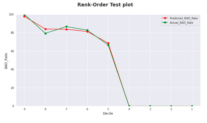
>>> aif.show_rank_measures(test_statistic='KS Test', model="XGB1", plot = False)
Display dataframe with below information:
    - Decile
    - Predicted_Bad_Rate
    - Actual_Bad_Rate

show_run_logs()

Displays all the run logs.

Param

None

Returns

Run logs as text/strings.

Example:

>>> aif.show_run_logs()

show_sample_entity_id(size=25, is_validation=True, key_var='ENTITY_ID')

Getting entities for given size from training or validation dataset

Parameters

• size – number of entity ids to get

• is_validation – True for validation data, otherwise training data

• key_var – Unique key column

Returns

list of entity ids for given size

show_saved_transformations(as_data_frame=False)

shows all the transformation ( UDT / OOB ) which are saved using self.save_transformations() API.

Parameters

as_data_frame – Options True/False. If False output is shown as python list else in data frame.

Returns

list of saved tranformations.

Example:

>>> aif.show_saved_transformations( as_data_frame = False )
>>> sample result will look like : ['Jump Bit Map', 'Time Series Clustering']

show_unused_attributes_in_model_group_metadata()

Attributes that are not enabled as metadata for model group creation, but do exist in the system.

Param

None

Returns

Attributes has not been enabled to use as model group metadata as pandas data frame.

update_transformations(include=None, exclude=None)

Update the transformation list manually to drop any transformations saved using self.save

Parameters

• include – provide the list of transformations to be included as python list.

• exclude – Or provide the list of transformations to be excluded as python list.

Note: use include/exclude, whichever is small/short.

Returns

successfully updates the saved transformation list.

Example:

>>> aif.update_transformations( exclude = [ 'Average Deposit' ] )

ofs_aif.aif_utility module

class aif_utility

Bases: object

The aif_utility contain reusable components mainly for the bulk activities. The list of below APIs interct with compliance studio without logging in to UI.

1. export models

2. get_objective_details

3. delete models

4. import_model_templates

5. get_models_summaries

6. fit_models

7. get_models_run_status

8. get_auc_summaries

9. publish models

10. get_reviewers_approvers_list

11. request_models_for_deployment

delete_models(mmg_url=None, id=None, version=None, notebookid=None, isobjective=True, headers=None)

This API is to delete the model or Objective from the MMG UI.

Parameters

• mmg_url – mmg service url. Ex: https://xyz.in.oracle.com:7002/cs

• id – modelid or objectiveid for model draft or Objective to delete

• version – Version of the model draft if modelid is passed.

• notebookid – notebookid of the model draft if modelid is passed.

• isobjective – True if Objective to be deleted, otherwise False for model.

• headers – API header, headers = {'workspace' : 'MMG', 'locale':'en_US','user':'MMGUSER'} Retrieve during the run time.

Returns

API response in json format.

Examples:

>>> #delete model draft
>>> headers = {'infodom' : 'MMG', 'locale':'en_US','user':'MMGUSER'}
>>> aif.delete_models(id='1623671951897', version=0, notebookid='dswaz2ea', isobjective=False, headers=headers)
>>>
>>> #delete Objective
>>> aif.delete_models(id='1628861985624', isobjective=true)

execution_status(mmg_url=None, headers=None, instanceid=None)

export_models(mmg_url=None, modelid=None, version=0, headers=None)

This API is called to dump the model to zip file on server. The dump’s path is configurable in DB table nextgenemf_config using variable FTPSHARE. Each model in mmg is associated with modelid and that can be found in table MMG_MODEL_MASTER

Parameters

• mmg_url – mmg service url. Ex: https://xyz.in.oracle.com:7002/cs

• modelid – modelid for model draft from MMG_MODEL_MASTER

• version – Version of the model draft from MMG_MODEL_MASTER

• headers – API header, headers = {'workspace' : 'MMG', 'locale':'en_US','user':'MMGUSER'} Retrieve during the run time.

Returns

API response in json format. zip file stored at path in format username_modelid_version.zip

Examples:

>>> #if mmg service is setting on different server
>>> headers = {'workspace' : 'MMG', 'locale':'en_US','user':'MMGUSER'}
>>> aif.export_models(mmg_url='https://xyz.in.oracle.com:7002/cs', modelid='1623671951897', version=0, headers=headers)
>>>
>>> #dynamic assignment of server details
>>> aif.export_models(modelid='1636975651884', version=0)
{'payload': {'modelid': '1636975651884', 'name': 'AMLES User Notebook', 'version': '0'}, 'messages': [{'severity': {'ordinal': 0}, 'params': [], 'key': 'COMMONOBJECT.GET_OBJECT_SUCCESSFUL'}], 'status': 'SUCCESS'}

fit_models(X=None, mmg_url=None, root_objectiveid='AMLES00002', type='DRAFT', links='training', isasync=True, headers=None, amles=True, **kwargs)

This API will execute the model’s draft

Parameters

• X – string or list of model groups

• mmg_url – mmg service url. Ex: https://xyz.in.oracle.com:7002/cs

• root_objectiveid – objective id of a parent Objective. Ex: AMLES/11000076_AC/SB, Objectiveid will be for AMLES.

• type – Summary for different type of models. options are DRAFT/PUBLISHED/ALL

• links – type of paragraphs to execute. options are training/scoring/default/experimentation Paragraphs to choose for different options would be set through mmg’s pipeline designer interface

• isasync – Boolean value(True/False). It decides if execute API should wait for pipeline execution or just trigger and exit. Default is True

• headers – API header, headers = {'workspace' : 'MMG', 'locale':'en_US','user':'MMGUSER'} Retrieve during the run time if not passed as a parameter

• **kwargs –

  any number of $ parameters to pass to notebook during run time. Make sure placeholders for capturing $ parameters are already configured in model’s draft. Parameters has to be passed in format param=value List of pre-defined params:

  • clsf_grid

  • ctrl_params

  • trainer_params

  • UDF

Returns

training status.

Examples:

>>> #if mmg service is setting on different server
>>> headers = {'workspace' : 'MMG', 'locale':'en_US','user':'MMGUSER'}
>>> aif.fit_models(mmg_url='https://xyz.in.oracle.com:7002/cs', root_objectiveid='1623321124592', headers=headers,
>>>            clsf_grid = clsf_grid, ctrl_params = ctrl_params, trainer_params=trainer_params, UDF=code,
>>>            unknown=code)
>>>
>>> #dynamic assignment of server details
>>> aif.fit_models(root_objectiveid='1623321124592', clsf_grid = clsf_grid,
>>>                        ctrl_params = ctrl_params, trainer_params=trainer_params,
>>>                        UDF=code, unknown=code)
>>>
>>> aif.fit_models(clsf_grid = clsf_grid,
>>>         ctrl_params = ctrl_params,
>>>         trainer_params=trainer_params,
>>>         date_range=[201603,201612],
>>>         enable_eda=False,
>>>         enable_feature_selection=False)
model_group     scenario_name               entity_type_name        segment_name    modelid         version     notebookid  model_status
110000085~CU        Rapid Movement of Funds     CUSTOMER        NA              1638972578712       0               dslapdma        COMPLETED
110000085~AC        Rapid Movement of Funds     ACCOUNT             NA                  1638972586251       0               dsWa77ka        COMPLETED

get_auc_summaries(model_group_include=None, model_group_exclude=None, top_n_models=1, algo=None, model_status='COMPLETED')

This API will return the AUC summary of the model which are successfully completed.

Parameters

• model_group_include – model groups to include

• model_group_exclude – model group to exclude

• top_n_models – display summary for top N models

• algo – getting an auc summary based on algorithm choosen. top_n_models will be disabled if algorithm is passed.

• model_status – summary for successfully completed models. Default is ‘COMPLETED’ Other options are ABORTED, FAILED, RUNNING and INPROGRESS

Returns

auc summary for top n models for different model groups.

Examples:

>>> #top 2 summaries for all model groups
>>> aif.get_auc_summaries(model_group_include=None, model_group_exclude=None, top_n_models=2)
>>>
>>> #top summary for given model group
>>> aif.get_auc_summaries(model_group_include=['110000085_CU_HNW'], model_group_exclude=None, top_n_models=1)
>>>
>>> #auc summary based on algo choosed
>>> aif.get_auc_summaries(model_group_include=['110000085_CU_HNW'], model_group_exclude=None, algo='XGB')
>>>
>>> aif.get_auc_summaries(model_group_include=None, model_group_exclude=None, top_n_models=1, algo=None)
MODEL_GROUP     Model       Validation      Mean_xval               Std_xval                    Median_xval         Best_xval               Worst_xval              Run1_R1F1               Run2_R1F2               Run3_R2F1               Run4_R2F2               Model_gid       Algo
110000085~CU        XGB1    1.0             0.9986468018760319      0.0006571289748328135   0.9988497824460646      0.9991455269648711      0.9977421156471271      0.9991455269648711      0.9985797182332696      0.9977421156471271      0.9991198466588596      XGB1        XGB
110000085~AC        XGB1    1.0             0.9986594359018259      0.0004855127066798656   0.9987125834282886      0.9991567750360583      0.9980558017146686      0.9989244772691153      0.9980558017146686      0.9991567750360583      0.998500689587462       XGB1        XGB

get_models_run_status(model_group_names=None, mmg_url=None, headers=None, debug_paragraphs=False)

This API will give a run status of the model groups triggered by fit_models api

Parameters

• model_group_names – String or list of model groups. If debug_paragraphs is True, single model group should be passed. Otherwise, debug output will only be displayed for the last model group in the list.

• mmg_url – mmg service url. Ex: https://xyz.in.oracle.com:7002/cs

• headers – API header, headers = {'workspace' : 'MMG', 'locale':'en_US','user':'MMGUSER'} Retrieve during the run time if not passed as a parameter

Debug_paragraphs

Boolean True/False. If True, Display the error occured at particular paragraph in the notebook

Returns

run status of all model groups. RUNNING or FAILED

Examples:

>>> #if mmg service is setting on different server
>>> headers = {'workspace' : 'MMG', 'locale':'en_US','user':'MMGUSER'}
>>> aif.get_models_run_status(mmg_url='https://xyz.in.oracle.com:7002/cs', headers=headers)
>>>
>>> #dynamic assignment of server details
>>> aif.get_models_run_status()
model_group     scenario_name           entity_type_name    segment_name    modelid         version notebookid      model_status
110000085~CU        Rapid Movement of Funds CUSTOMER                NA                  1638972578712       0           dslapdma    COMPLETED
110000085~AC        Rapid Movement of Funds ACCOUNT             NA              1638972586251       0           dsWa77ka    COMPLETED

get_models_summaries(mmg_url=None, root_objectiveid='AMLES00002', type='DRAFT', headers=None)

This API will return summary for model’s hiererachy under root or main objective.

Parameters

• mmg_url – mmg service url. Ex: https://xyz.in.oracle.com:7002/cs

• root_objectiveid – objective id of a parent Objective. Ex: AMLES0002, Objectiveid for parent folder.

• type – Summary for different type of models. options are DRAFT/PUBLISHED/ALL

• headers – API header, headers = {'workspace' : 'MMG', 'locale':'en_US','user':'MMGUSER'} Retrieve during the run time if not passed as a parameter

Returns

model’s summary in json format.

Examples:

>>> #if mmg service is setting on different server
>>> headers = {'workspace' : 'MMG', 'locale':'en_US','user':'MMGUSER'}
>>> aif.get_models_summaries(mmg_url='https://xyz.in.oracle.com:7002/cs', root_objectiveid='1623321124592', headers=headers)
>>>
>>> #dynamic assignment of server details
>>> aif.get_models_summaries(root_objectiveid='1623321124592')

get_objective_details(mmg_url=None, headers=None)

This API is called to get all objectives and their ids under root directory

Parameters

• mmg_url – mmg service url. Ex: https://xyz.in.oracle.com:7002/cs

• headers – API header, headers = {'workspace' : 'MMG', 'locale':'en_US','user':'MMGUSER'} Retrieve during the run time.

Returns

API response in json format.

Examples:

>>> #if mmg service is setting on different server
>>> headers = {'workspace' : 'MMG', 'locale':'en_US','user':'MMGUSER'}
>>> aif.get_objective_details(mmg_url='https://xyz.in.oracle.com:7002/cs', headers=headers)
>>>
>>> #dynamic assignment of server details
>>> aif.get_objective_details()
{'payload': [{'description': 'Admin Activity for AIF4AML', 'label': 'AIF Admin', 'value': 'AIF0000018'},
{'description': 'Batch Framework for AIF4AML', 'label': 'AIF Batch Framework', 'value': 'AIF0000005'},
{'description': 'Batch Framework for AIF4AML', 'label': 'AIF Batch Framework/Supervised ML', 'value': 'AIF0000006'},
{'description': 'Batch Framework for AIF4AML', 'label': 'AIF Batch Framework/Supervised ML/Big Data', 'value': '1628752209023'},
{'description': 'Batch Framework for AIF4AML', 'label': 'AIF Batch Framework/Supervised ML/Graph Analytics', 'value': '1628752791075'},
{'description': 'Batch Framework for AIF4AML', 'label': 'AIF Batch Framework/Supervised ML/Event Processing', 'value': 'AIF0000008'},
{'description': 'Batch Framework for AIF4AML', 'label': 'AIF Batch Framework/Supervised ML/Historical Data', 'value': 'AIF0000009'},
{'description': 'Batch Framework for AIF4AML', 'label': 'AIF Batch Framework/Supervised ML/Scoring Data', 'value': 'AIF0000010'},
{'description': 'Batch Framework for AIF4AML', 'label': 'AIF Batch Framework/Supervised ML/Ongoing Model Validation', 'value': 'AIF0000011'},
{'description': 'Batch Framework for AIF4AML', 'label': 'AIF Batch Framework/Supervised ML/Ongoing Model Validation/Annual', 'value': 'AIF0000012'},
{'description': 'Batch Framework for AIF4AML', 'label': 'AIF Batch Framework/Supervised ML/Ongoing Model Validation/Monthly', 'value': 'AIF0000013'},
{'description': 'Batch Framework for AIF4AML', 'label': 'AIF Batch Framework/Supervised ML/Ongoing Model Validation/Monthly/Model Drift', 'value': 'AIF0000014'},
{'description': 'Batch Framework for AIF4AML', 'label': 'AIF Batch Framework/Supervised ML/Ongoing Model Validation/Monthly/Data Quality', 'value': 'AIF0000015'},
{'description': 'Batch Framework for AIF4AML', 'label': 'AIF Batch Framework/Unsupervised ML', 'value': 'AIF0000007'},
{'description': 'Batch Framework for AIF4AML', 'label': 'AIF Batch Framework/Unsupervised ML/Historical Data', 'value': 'AIF0000016'},
{'description': 'Batch Framework for AIF4AML', 'label': 'AIF Batch Framework/Unsupervised ML/Scoring Data', 'value': 'AIF0000017'},
{'description': 'AIF Data Aggregation in Big Data', 'label': 'AIF Big Data', 'value': 'AIF0000020'},
{'description': 'PGX for AIF4AML', 'label': 'AIF Graph Analytics', 'value': 'AIF0000019'}, {'description': 'Supervised ML for AIF4AML', 'label': 'AIF Supervised ML', 'value': 'AIF0000001'},
{'description': 'Supervised ML for AIF4AML', 'label': 'AIF Supervised ML/AIF', 'value': 'AIF0000002'}, {'description': 'Supervised ML for AIF4AML', 'label': 'AIF Supervised ML/AIF/LOB2', 'value': '1629795499565'},
{'description': 'Unsupervised ML for AIF4AML', 'label': 'AIF Unsupervised ML', 'value': 'AIF0000003'}, {'description': 'Unsupervised ML for AIF4AML', 'label': 'AIF Unsupervised ML/AIF', 'value': 'AIF0000004'},
{'description': 'Unsupervised ML for AIF4AML', 'label': 'AIF Unsupervised ML/AIF/MODEL_GROUP_X', 'value': '1629872123411'}, {'description': 'AMLES Models', 'label': 'AMLES', 'value': 'AMLES00002'},
{'description': 'AMLES Models', 'label': 'AMLES/test', 'value': '1629879466333'}, {'description': 'AMLES Models', 'label': 'AMLES/110000085~CU~HNW', 'value': '1629883248308'},
{'description': 'AMLES Models', 'label': 'AMLES/110000085~AC~HH', 'value': '1629883251738'}, {'description': 'AMLES Models', 'label': 'AMLES/110000085~CU~HH', 'value': '1629883255336'},
{'description': 'AMLES Models', 'label': 'AMLES/110000085~AC~HNW', 'value': '1629883258686'}, {'description': 'AMLES Models', 'label': 'AMLES/110000086~AC~SB', 'value': '1629883262123'},
{'description': 'AMLES Application', 'label': 'AMLES Admin', 'value': 'AMLES00001'}, {'description': 'Batch Framework for AMLES', 'label': 'AMLES Batch Framework', 'value': 'AMLES00003'},
{'description': 'Batch Framework for AMLES', 'label': 'AMLES Batch Framework/ECM Update', 'value': 'AMLES00004'}, {'description': 'Batch Framework for AMLES', 'label': 'AMLES Batch Framework/Load Events', 'value': 'AMLES00005'},
{'description': 'Batch Framework for AMLES', 'label': 'AMLES Batch Framework/Update Event Labels', 'value': 'AMLES00006'}], 'messages': 'SUCCESS', 'status': 'SUCCESS'}

get_reviewers_approvers_list(mmg_url=None, headers=None)

This API will return available list of approvers and reviewers.

Parameters

• mmg_url – mmg service url. Ex: https://xyz.in.oracle.com:7002/cs

• headers – API header, headers = {'workspace' : 'MMG', 'locale':'en_US','user':'MMGUSER'} Retrieve during the run time if not passed as a parameter

Returns

list of approvers and reviewers

Examples:

>>> aif.get_reviewers_approvers_list()
code        name                group_type
MDLAPPR     Modeling Approver       Approvers
MDLREV      Modeling Reviewer       reviewers

import_model_templates(objectives=None, mmg_url=None, filename=None, filepath=None, headers=None, overwrite=False, amles=True)

This API will create the objectives in MMG by taking model group names as an input and also import model drafts to respective objectives.

Parameters

• objectives – It can be a dict or list of dictionaries of an objectives hierarchy. if None, will create the model’s group from self.select_amles_models_granularity

• mmg_url – mmg service url. Ex: https://xyz.in.oracle.com:7002/cs

• filename – filename of model’s draft in zip format.

• filepath – Path where zip dump is put

• headers – API header, headers = {'workspace' : 'MMG', 'locale':'en_US','user':'MMGUSER'} Retrieve during the run time if not passed as a parameter

• overwrite – if True, it will delete the lowest level objective and then recreate with updated notebook.

Returns

API response in json format.

Examples:

>>> #if mmg service is setting on different server
>>> headers = {'workspace' : 'MMG', 'locale':'en_US','user':'MMGUSER'}
>>> aif.import_model_templates(mmg_url='https://xyz.in.oracle.com:7002/cs', filename='AIFQA2_1627313165462_0.zip', headers=headers)
>>>
>>> #dynamic assignment of server details
>>> aif.import_model_templates()
>>>
>>> #single objective
>>> input = {"1":{
>>>         "name": "AMLES",
>>>            "desc" : "AMLES Models"},
>>>        "2": {
>>>            "name": 'scenario_entity',
>>>            "desc": 'scenario name and entity name'},
>>>        "3": {
>>>            "name": 'segment',
>>>            "desc": 'segment name'}}
>>>
>>> #delete an existing copy and re-import an updated dump file
>>> aif.import_model_templates(objectives=input, filename='MMG_1623671951897_0.zip', overwrite=True)
>>> aif.import_model_templates(overwrite=True)
{'1': {'name': 'AMLES', 'desc': 'AMLES Models'}, '2': {'name': '110000085~CU', 'desc': 'Rapid Movement of Funds~CUSTOMER'}}
Model group 110000085~CU already exist
overwrite flag is True.....
{'payload': 'Successfully deleted model 1637574613955 with version 1.  Successfully deleted objective 1637574608641.  ', 'messages': 'SUCCESS', 'status': 'SUCCESS'}
{'payload': '{"modelid":"1638972578712","name":"AMLES User Notebook","objectiveid":"1638972572281","objectives":[{"name":"110000085~CU","id":"1638972572281"}],"version":"0"}', 'status': 'SUCCESS'}
{'1': {'name': 'AMLES', 'desc': 'AMLES Models'}, '2': {'name': '110000085~AC', 'desc': 'Rapid Movement of Funds~ACCOUNT'}}
Model group 110000085~AC already exist
overwrite flag is True.....
{'payload': 'Successfully deleted model 1637053489976 with version 0.  Successfully deleted objective 1637053485055.  ', 'messages': 'SUCCESS', 'status': 'SUCCESS'}
{'payload': '{"modelid":"1638972586251","name":"AMLES User Notebook","objectiveid":"1638972580370","objectives":[{"name":"110000085~AC","id":"1638972580370"}],"version":"0"}', 'status': 'SUCCESS'}
True

publish_models(mmg_url=None, headers=None, model_group_include=None, model_group_exclude=None, scenario_include=None, scenario_exclude=None, modelname=None, modeldesc='Model for risk', techniqueid=None, runversion=0, model_status='COMPLETED')

This API will publish the model.

Parameters

• mmg_url – mmg service url. Ex: https://xyz.in.oracle.com:7002/cs

• headers – API header, headers = {'workspace' : 'MMG', 'locale':'en_US','user':'MMGUSER'} Retrieve during the run time if not passed as a parameter

• model_group_include – model groups to include

• model_group_exclude – model group to exclude

• scenario_include – scenarios to include

• scenario_exclude – scenarios to exclude

• modelname – name of the model to publish

• modeldesc – description for the model to publish

• techniqueid – technique id to be published. Ex: ‘XGB1’, ‘XGB2_ne20_fiN_rtT’ if it is not passed, then best model will be published

• runversion – version of the model to publish

• model_status – summary for successfully completed models. Default is ‘COMPLETED’ Other options are ABORTED, FAILED, RUNNING and INPROGRESS

Returns

publish model to mmg and return successful message

Examples:

>>> #publish model based on technique
>>> aif.publish_models(model_group_include=['110000086_AC'], scenario_exclude=['Rapid Movement of Funds'],
>>>                    modeldesc='Model for risk', techniqueid='XGB1')
>>>
>>> #publish model when technique is not passed
>>> aif.publish_models(model_group_include=['110000086_AC'], scenario_exclude=['Rapid Movement of Funds'])
>>>
>>> aif.publish_models(techniqueid = 'XGB1')
model_group     scenario_name               entity_type_name        segment_name    modelid         version     publish_version         model_status
110000085~CU        Rapid Movement of Funds CUSTOMER                NA                  1638972578712       0           1                   PUBLISHED
110000085~AC        Rapid Movement of Funds ACCOUNT             NA              1638972586251       0               1                       PUBLISHED

request_models_for_deployment(mmg_url=None, headers=None, model_group_include=None, model_group_exclude=None, scenario_include=None, scenario_exclude=None, approvers=None, reviewers=None, comments='default comment - Kindly approve', requesttype='REQUEST_ACCEPT_PROMOTE', model_status='PUBLISHED')

This API will publish the model.

Parameters

• mmg_url – mmg service url. Ex: https://xyz.in.oracle.com:7002/cs

• headers – API header, headers = {'workspace' : 'MMG', 'locale':'en_US','user':'MMGUSER'} Retrieve during the run time if not passed as a parameter

• model_group_include – model groups to include

• model_group_exclude – model group to exclude

• scenario_include – scenarios to include

• scenario_exclude – scenarios to exclude

• approvers – valid approver’s group

• reviewers – valid reviewer’s group

• comments – comment for requested model.

• requesttype –

  type of request. Default is ‘REQUEST_ACCEPT_PROMOTE’ i.e Request for model acceptance and promotion to production Other options are:-

  1. REQUEST_MODEL_ACCEPT: Request for model acceptance

  2. REQUEST_ACCEPT_PROMOTE : Request for Model Acceptance and Promotion to production

  3. REQUEST_PROMOTE : Request for Promotion to production for already accepted models

  4. REQUEST_CHAMP_GLOBAL : Request for global champion

  5. REQUEST_CHAMP_LOCAL : Request for local champion

• model_status – request model for successful published draft. Default is “PUBLISHED”

Returns

request model for review and approval.

Examples:

>>> aif.request_models_for_deployment(model_group_include=['110000086_AC'],
>>>                         scenario_exclude=['Rapid Movement of Funds'],
>>>                         approvers='MDLAPPR',
>>>                         reviewers='MDLAPPR')
model_group     scenario_name               entity_type_name        segment_name    modelid         version     approvers   reviewers       comment_version model_status
110000085~CU        Rapid Movement of Funds CUSTOMER            NA              1638972578712       0               MDLAPPR     MDLREV          1               REQUESTED
110000085~AC        Rapid Movement of Funds ACCOUNT             NA              1638972586251       0               MDLAPPR     MDLREV          1               REQUESTED

ofs_aif.amles module

class amles(connect_with_default_workspace=True)

Bases: ofs_aif.supervised.supervised

This class amles is a special use case of supervised learning for anti-money laundering for event scoring (AMLES)

add_model_groups(model_group_name=None)

Create segmentation (model group) for AMLES

Parameters

model_group_name – Unique name for the model group. Only alphanumeric character set including underscore, hyphen and space are allowed

Returns

successful message on successfully creating the model groups in AIF system.

Examples:

>>> input_pdf = pd.DataFrame({'MODEL_GROUP_NAME'   : ["100087_AC"],
>>>                         'ENTITY_NAME'         : ["AMLES"],
>>>                         'ATTRIBUTE_NAME'      : ["AMLES"],
>>>                         'ATTRIBUTE_VALUE'     : ["AMLES"],
>>>                         'LABEL_FILTER'        : ["AMLES"],
>>>                         'FEATURE_TYPE_FILTER' : ["AMLES"]
>>>                         })
>>>
>>> supervised.add_model_groups(self, input_pdf )

create_evented_data(scenario_code=None, entity_type_code=None, segment_code=None, date_range=None, osot_date_range=None)

This API prepares amles data using amles.create_evented_data from table fsi_es_event_input and stores them in AIF class members self.B_DF for in-time and self.B_DF_OSOT for out-time (osot). SCENARIO_CODE, ENTITY_TYPE_CODE and SEGMENT_CODE make a unique filter to get data from table.

Parameters

• scenario_code – Unique Scenario code corresponding to table column V_SCENARIO_CODE

• entity_type_code – Unique Entity type columns corresponding to table column V_ENTITY_TYPE_CODE

• segment_code – Unique Entity type columns corresponding to table column V_SEGMENT_CODE

• date_range – From and To Date for OSIT ( Model Build ) data set in YYYYMM format or YYYYMMDD as numeric data type. Example: date_range = [201501, 201512] Example: date_range = [20150114, 20151231]

• osot_date_range – From and To Date for OSOT Validation data set in YYYYMM format as numeric data type Example: osot_date_range = [201601, 201612]

Returns

osit and osot data is stored in class members for further references.

Example:

>>> amles.create_evented_data( scenario_code='110000086', entity_type_code='AC', segment_code='SB',
>>>                  date_range=[201603,201612], osot_date_range=[201701,201702])
create amles data preparation successful...
True

create_modeling_dataset(X=None, osot=False)

This API converts any new AMLES data into modelling data by applying all the transformations recorded during training process for unsupervised.

Parameters

• X – AMLES input data as pandas data frame.

• osot – Boolean flag to indicate data set type ( in-time or out-time (OSOT) ). Set to False always while prediction.

Returns

AMLES stage 2 created data is saved inside the class object.

Example:

>>> amles.create_modeling_dataset( X )

get_evented_data(osot=False)

Get amles in-time/out-time(osot) data as pandas data frame.

Parameters

osot – Boolean flag to indicate data set type ( in-time or out-time (OSOT) ). False : (default) For in-time data set. ( Model build dataset ) True : For OSOT dataset.

Returns

osit/osot data as pandas data frame.

Example:

>>> B_OSIT_PDF  = self.get_evented_data();
Data dimension  : 41544 x 8
>>> B_OSOT_PDF  = self.get_evented_data(osot = True);
OSOT dataset is None

predict(X=None, key_column='EVENT_ID', model_group_name=None, model_group_scenario_name=None, fic_mis_date=None, batch_run_id=None, threshold=0.7, return_score=False, debug=False)

Test scoring interactively by connecting to production like schema before scheduling it as batch process in real production. Same sandbox can also be used for the scoring purpose. In this case sandbox schema should have scoring related input and output tables. All run time parameters expected during scoring batch should be set in studio paragraph for testing purpose.

Parameters

• X – Stage 2 transformed new data as pandas data frame. default is None

• key_column – Identity column

• model_group_name – Name of the deployed model group.

• model_group_scenario_name – Name of the deployed model group scenario. Always None for AMLES

• fic_mis_date – AAI FIC MIS Date used in the batch execution.

• batch_run_id – AAI Batch Run ID for the execution

• threshold – Threshold to generate events for ECM. default 0.7

• return_score – Boolean flag. If set to True scoring result is returned as panadas data frame to the caller. Default is False, and which is real production use case.

• debug – Boolean(True/False). If set to True, debug mode is on

Returns

Returns output scores as pandas data frame.

Examples:

>>> score_pdf_list = self.predict(X = Stage_2_OSOT_pdf,
>>>                 key_column = 'ENTITY_ID'
>>>                 model_group_name = '110000085_CU',
>>>                 model_group_scenario_name = None,
>>>                 fic_mis_date = date.today(),
>>>                 batch_run_id = 'RRF_ICC_BATCH_123',
>>>                 threshold = 0.5,
>>>                 return_score = True,
>>>                 debug = True )
Returns output scores as pandas data frame

select_model_granularity(scenarios_include=None, scenarios_exclude=None, entities_include=None, entities_exclude=None, segments_include=None, segments_exclude=None, models_at_segment_level=True)

API is used to select different scenarios or entities or segments or their combinations for model group creation. User can choose either 2-level or 3-level model group creation depending on the parameter models_at_segment_level.

Parameters

• scenarios_include – Scenarios to be a part of model group creation

• scenarios_exclude – Scenarios not to be a part of model group creation

• entities_include – Entities to be a part of model group creation

• entities_exclude – Entities not to be a part of model group creation

• segments_include – Segments to be a part of model group creation

• segments_exclude – Segments not to be a part of model group creation

• models_at_segment_level – 3-level or segment level group creation if it is True. The flag has has to be made True if either segment include or exclude is considered. Otherwise, it would ignore the inputs for segment include or exclude.

:Note

Inputs passed to scenarios, entities or segments are case insensitive.

Returns

combination of model group codes with their descriptions.

Examples:

>>> #2-level : models_at_segment_level = False
>>> amles.select_model_granularity(scenarios_include=['Rapid Movement of Funds'],
>>>                         scenarios_exclude=None,
>>>                         entities_include=['ACCOUNT'],
>>>                         entities_exclude=None,
>>>                         segments_include=None,
>>>                         segments_exclude=None,
>>>                         models_at_segment_level = False)
MODEL_GROUP_NAME    MODEL_GROUP_DESCRIPTION
110000085_AC            Rapid Movement of Funds_ACCOUNT
>>> #3-level : models_at_segment_level = True
>>> amles.select_model_granularity(scenarios_include=['Rapid Movement of Funds'],
>>>                         scenarios_exclude=None,
>>>                         entities_include=['ACCOUNT'],
>>>                         entities_exclude=None,
>>>                         segments_include=None,
>>>                         segments_exclude=None,
>>>                         models_at_segment_level = True)
MODEL_GROUP_NAME         MODEL_GROUP_DESCRIPTION
110000085_AC_HH              Rapid Movement of Funds_ACCOUNT_Household
110000085_AC_HNW         Rapid Movement of Funds_ACCOUNT_High Net Worth

show_scenarios(show_scenarios=True, show_entities=False, show_segments=False)

View Available AMLES scenarios/entity/segments or Displays all the scenarios available in table fsi_es_event_input

Parameters

• show_scenarios – display scenario code and names. Default True

• show_entities – display entity code and names. Default False

• show_segments – display segment code and names. Default False

Returns

pandas dataframe with scenarios codes and names, entity code and names, segment code and names

Example:

>>> amles.show_scenarios(show_scenarios=True,
>>>                    show_entities=False,
>>>                    show_segments=False)
V_SCENARIO_CODE      V_SCENARIO_NAME
110000085            Rapid Movement of Funds
110000086            CIB - Product Utilization

>>> aif.show_scenarios(show_scenarios=True,
>>>                    show_entities=True,
>>>                    show_segments=True)
V_SCENARIO_CODE     V_SCENARIO_NAME         V_ENTITY_TYPE_CODE      V_ENTITY_TYPE   V_SEGMENT_CODE  V_SEGMENT_NAME
110000085       Rapid Movement of Funds         CU              CUSTOMER            HNW             High Net Worth
110000085       Rapid Movement of Funds         AC              ACCOUNT                 CORP            Corporate
110000085       Rapid Movement of Funds         AC              ACCOUNT                 HH          Household
110000085       Rapid Movement of Funds         CU              CUSTOMER            HH              Household
110000085       Rapid Movement of Funds         AC              ACCOUNT                 HNW         High Net Worth
110000086       CIB - Product Utilization   AC                  ACCOUNT                 SB          Small Business

ofs_aif.supervised module

class supervised(connect_with_default_workspace=True)

Bases: ofs_aif.aif.aif, ofs_aif.aif_utility.aif_utility

The supervised class contain methods required for supervised learning. It inherits methods from the aif and aif_utility classes.

annual_model_validation(X=None, y=None, B_PDF=None, NB_PDF=None, osot_end_month=None, model_group_name=None, model_group_scenario_name=None, model_id_list=['Best'], printrs=False, performance_metrics_list=['ROC Curve'])

To evaluate the performance of the Model Annually. This API makes use of the Deployed Modelor the Selected Model for the particular Definition ID. The metrics is then generated on the new data or OSOT data to validate the performance of the Model. It supports the following flavors in which data can be provided:

1. X and y -> OSOT data available at each Entity level along with labels.

2. B_PDF and NB_PDF -> Behavioral and Non-behavioral dataset on which the transformations(saved during Training process) will be applied to generate data at each entity level.

3. osot_end_month -> The data will be picked from the AIF tables to generate time-series data and then the modeling dataset from osot_end_month - osit_month_range to osot end month. If osot_end_month is None, data will be picked from max(month) - osit_month_range to the max(month)

NOTE:

At a time, only one of the above options can be used.

Parameters

• X – New Data or OSOT data which will be used to validate the Model

• y – Label in the new dataset.

• B_PDF – Behavioral Dataframe

• NB_PDF – Non-behavioral dataframe

• osot_end_month – OSOT end month in the format YYYYMMDD

• model_group_name – Model group for which the validation has to be performed

• model_group_scenario_name – Model group Scenario for which the validation has to be performed

• model_id_list – List of Model ids for which Model has to be evaluated.

• printrs – (True/False) to print the output. If set to True, will print AUC Change and PSI.

• performance_metrics_list –

  List of performance metrics on which the Model has to be evaluated. Available Metrics:

  • Kappa Curve

  • F1 Curve

  • PR Curve

  • ROC Curve

  • Prediction Density

  • Confusion Matrix:Kappa

  • AUC Change

  • PSI

Returns

Plot or metric depending the types of performance metric chosen

Examples:

>>> result_dict = aif.annual_model_validation(X=X_osot, y=y_osot, model_group_name='LOB1',
>>>             model_group_scenario_name=None, model_id_list='Deployed', printrs=False ,
>>>             performance_metrics_list='ROC Curve~Prediction Density~PR Curve~Confusion Matrix~PSI')
>>>
>>> result_dict = aif.annual_model_validation(B_PDF=B_PDF, NB_PDF=NB_PDF, model_group_name='LOB1',
>>>             model_group_scenario_name=None, model_id_list='Deployed', printrs=False,
>>>             performance_metrics_list='F1 Curve~Kappa Curve~PR Curve~Confusion Matrix')
>>>
>>> result_dict = aif.annual_model_validation(osot_end_month=None, model_group_name='LOB1',
>>>             model_group_scenario_name=None, model_id_list='Deployed', printrs=False,
>>>             performance_metrics_list='ROC Curve~Prediction Density~PR Curve~Confusion Matrix')

create_modeling_dataset_for_osot(B_OSOT=None, NB=None, osot=True)

The API converts any new/osot behavioral data into modeling dataset by applying all the transformations recorded during in-time data conversion.

Parameters

• B_OSOT – out-time (OSOT) behavioral data as pandas data frame.

• NB – Non behavioral data as pandas data frame.

Returns

modeling dataset created and saved inside the class object.

Example:

>>> aif.create_modeling_dataset_for_osot(B_OSOT_PDF, NB_PDF)
Behavioral Data Dimension     :  [11160, 9]
Non Behavioral Data Dimension :  [12000, 3]
Applying Transformation  :  Average Deposit
Applying Transformation  :  Time Series Clustering
Applying Transformation  :  Jump Bit Map
Transformation successful...
Stage 2 creation successful...
True

create_time_series_dataset(date_range=None, osot_date_range=None)

It’s a One Time Mandatory API Call. This API creates time series data for the subset of date range. create_time_series_dataset persists data in oracle tables, hence there’s no need to call this API every time in studio unless there is a change in date range filters.

Parameters

• date_range – From and To Date for in-time (Model Build) data set in YYYYMM format as numeric data type.

• osot_date_range – From and To Date for OSOT Validation data set in YYYYMM format as numeric data type

Returns

Permanent save of data in Oracle tables, unless API is re-executed. This helps in avoiding data re-calculations due to studio session invalidations. Shows successful message on completion.

Example:

>>> aif.create_time_series_dataset(date_range=[201501, 201612], osot_date_range=[201701, 201812])
Create time series data successful...
True
>>> aif.create_time_series_dataset(date_range=[201501, 201612])
Create time series data successful...
True

data_quality_data_preparation(X=None, B_PDF=None, NB_PDF=None, osot_end_month=None, model_group_name=None, model_group_scenario_name=None)

Data quality checks on the input data. This API prepares the data for different quality checks on input data. Returned object would be passed to an API data_quality_report. It supports the following flavors in which data can be provided:

1. X -> OSOT data available at each Entity level along with labels.

2. B_PDF and NB_PDF -> Behavioral and Non-behavioral dataset on which transformations(saved during Training process) will be applied to generate data at each entity level.

3. osot_end_month -> The data will be picked from the AIF tables to generate modeling data and then modeling dataset from osot_end_month - osit_month_range to osot end month. If osot_end_month is None, data will be picked from max(month) - osit_month_range to the max(month).

NOTE:

At a time, only one of the above options can be used.

Parameters

• X – New Data or OSOT data which will be used to validate the Model

• B_PDF – Behavioral Dataframe

• NB_PDF – Non-behavioral dataframe

• osot_end_month – osot end month in the format YYYYMMDD

• model_group_name – Model group for which the validation has to be performed

• model_group_scenario_name – Model group Scenario for which the validation has to be performed

Returns

Object of the class DataQualityCheck from module ofs_auto_ml.utils.data_quality_checks.

Examples:

>>> dq_object = aif.data_quality_data_preparation(X=X_osot, model_group_name='LOB1',
>>>                                               model_group_scenario_name=None)

data_quality_report(dq_obj, variable_type=['continuous', 'categorical'], measure=['summary', 'variance', 'correlation', 'scatterplot'], feature_include=None, feature_exclude=None)

Generates data quality report for different quality checks:

1. Summary for categorical features

2. summary for continuous features

3. variance for continuous features

4. correlation matrix

5. scatter plot

It supports the following flavors in which data can be provided:

1. dq_obj -> Object returned from API data_quality_data_preparation object of the class DataQualityCheck from module ofs_auto_ml.utils.data_quality_checks

2. variable_type -> continuous or categorical summary

3. measure -> metrics/plots to display on data quality report

Parameters

• dq_obj – New Data or OSOT data which will be used to validate the Model

• variable_type – summary for continuous or categorical features.

• measure – output to display in data quality report

• feature_include – List of features to be included.

• feature_exclude – List of features to be excluded.

Returns

summary report for various data quality checks

Examples:

>>> aif.data_quality_report(dq_object, variable_type='continuous', measure='summary')
>>>
>>> aif.data_quality_report(dq_object, variable_type='continuous', measure='variance')
>>>
>>> aif.data_quality_report(dq_object, variable_type='categorical', measure='summary')
>>>
>>> aif.data_quality_report(dq_object, variable_type='continuous', measure='correlation')
>>>
>>> aif.data_quality_report(dq_object, variable_type='continuous', measure='scatterplot')

fit(clsf_grid=None, ctrl_params=None, trainer_params=None, X=None, y=None, X_osot=None, y_osot=None, feature_include=None, feature_exclude=None, feature_must_include=None, univariate_selector=None, multivariate_selector=None, key_column='ENTITY_ID')

Fit classification models

• Model fitting is a measure of how well a machine learning model generalizes to similar data to that on which it was trained.

• A model that is well-fitted produces more accurate outcomes.

• Compare the outcomes to real, observed values of the target variable to determine their accuracy.

Parameters

• clsf_grid – Classifier grid for modelling

• ctrl_params – Control parameters for modelling.

• trainer_params – Trainer control parameters for modelling.

• X – Input dataframe

• y – Input target data (binary: should be populated with 0 or 1. 1 indicating the minority class)

• X_osot – OSOT validation dataframe (Default: None)

• y_osot – OSOT validation target data (Default: None)

• feature_include – List of features to include while fitting the model (Default: None)

• feature_exclude – List of features to exclude while fitting the model (Default: None)

• feature_must_include – List of features (Default: None)

• univariate_selector – Key-Value pairs indicating the uni-variate feature selection method along with the respective paramters (Default: None).

• multivariate_selector – Key-Value pairs indicating the multivariate feature selection method along with the respective paramters (Default: None).

• key_column – Identity column

Returns

Examples:

Sample clsf_grid, ctrl_params, trainer_params
clsf_grid = [
         {"models": ["WOELR", "LR", "ADB", "MLP", "XGB", "GB", "RF"]},

         {"models": ["XGB"],
             "params":{'n_estimators': range(10,20)},
             "ctrls": {"feature_include": None}},
         {"models": ['NB']}
        ]

ctrl_params = {
        "drop_col_nan_pct"                  : 0.2,
        "drop_col_variance_thrsh"           : 0,
        "find_linear_combos"                : True,
        "min_col_uniq_lvls"                 : 2,
        "max_col_uniq_lvls"                 : 100,
        "auto_data_partition"               : True,
        "min_validation_data_pct"           : 0.2,
        "max_cv_runs_per_model"             : 4,
        "max_cv_folds_per_repeat"           : 2,
        "min_minority_obs_fold"             : 30,
        "max_oversample_ratio"              : 0,
        "auto_univariate_feature_selector"  : True,
        "auto_multivariate_feature_selector": True,
        "calibrate_scores"                  : True
       }

trainer_params = {
          "validation_type"    : "OSIT",
          "xval"               : "auto",
          "sampling"           : "stratified",
          "holdout_validation" : "auto",
          "n_folds"            : 10,
          "repeats"            : 2
         }

>>> aif.fit(clsf_grid=clsf_grid,
>>>         ctrl_params=ctrl_params,
>>>         X=modeling_pdf,
>>>         y=y)
>>>
>>> aif.fit(clsf_grid=clsf_grid,
>>>         ctrl_params=ctrl_params,
>>>         X=modeling_pdf,
>>>         y=y,
>>>         feature_include=['feature_1', 'feature_5'],
>>>         multivariate_selector={"method": "varclus",
>>>                                "min_proportion": 0.75})
>>>
>>> aif.fit( clsf_grid = clsf_grid,
>>>         ctrl_params = ctrl_params,
>>>         trainer_params = trainer_params,
>>>         X = modeling_pdf,
>>>         y = y,
>>>         X_osot = modeling_OSOT_pdf,
>>>         y_osot = y_osot,
>>>         feature_include=None,
>>>         feature_exclude=None,
>>>         feature_must_include=None,
>>>         univariate_selector=None,
>>>         multivariate_selector=None)
Display running log output

get_case_data_and_sar_classification(p_from_date, p_to_date, CRR_conn, ECM_conn)

get_drift_history(model_group_name=None, model_group_scenario_name=None, monitoring_technique='MD', look_back_months=5)

This API is used in Monthly model validation for retrieving drift history for different metrics. The drift history is retrieved for both monitoring techniques i.e. CDBD and MD

Parameters

• model_group_name – Name of the model group for which drift history to be retrieved.

• model_group_scenario_name – Name of the model group scenario for which drift history to be retrieved.

• monitoring_technique – List of monitoring techniques: - Confidence Distribution Batch Detection Method (CDBD) or - Margin density (MD)

• look_back_months – Number of previous months for which drift history to be retrieved. Default to 5 months

Returns

pandas dataframe

Examples:

>>> aif.get_drift_history(model_group_name='LOB2')
>>>
>>> aif.get_drift_history(model_group_name='LOB2', look_back_months=3)

get_investigation_data(p_from_date, p_to_date, p_cust_sar, p_acct_sar, ECM_conn)

get_nearest_neighbors_graph(X, nearest_neighbors=3)

Get the historical SARs if matched exactly or nearly match or no match based on the graph features

Parameters

• X – Input prod data (Modeling data with graph features ended with *_EMBED)

• nearest_neighbors – [Optional] integer value to get number of nearest SARs case information needed. - Exact Match: if graph features are matched exactly, CASE information for those matched entities will be retrieved. - Nearest Match: Based on the cosine similarity between graph features, nearest similar cases will be retrieved.

Returns

Dict with case information.

Note: Using internally while predict

get_nearest_neighbors_tsc(X, nearest_neighbors=3)

Get the historical SARs if matched exactly or nearly match or no match based on the RLEs calculated for features of time series

Parameters

• X – Input modeling data with TS features (ended with *_CLIP and *_TREND)

• nearest_neighbors –

  [Optional] integer value to get number of nearest SARs case information needed. For each TS feature, nearest SAR’s will be returned.

  • Exact Match: if TS and rle matched exactly, then only matched entities will be returned

  • Nearest Match: if any TS feature is matched, then Euclidean distance between rle’s will be calculated to get the nearest SARs for filtered records on TS value

  • No Match: if TS feature is not matched, rle will be calculated for complete data set and nearest cases will be retrieved.

Returns

Dict with case information.

Note: Using internally while predict

get_sar_data(p_from_date, p_to_date, CRR_conn)

get_time_series_dataset(osot_end_month=None)

This API loads time series data created using aif.create_time_series_dataset and stores them in AIF class members.

Parameters

osot_end_month – Default value is None. This parameter is applicable only during scoring to get latest month data. Not applicable for sandbox.

Returns

Behavioral and Non-Behavioral data is stored in class members for further references.

Example:

>>> aif.get_time_series_dataset()
Get time series data successful...
True

import_model_template(meta_data_df=None, model_group_scenario=None, overwrite=False)

This API will create the objectives in MMG by taking model group metadata as an input and also imports model drafts to respective objectives.

Parameters

• meta_data_df – Same as the one created for adding model groups.

• model_group_scenario – Model group scenario name as string.

• overwrite – If True Model Templates will be overwritten.

Root_objectiveid

Objectiveid of the parent folder. Ex: AIF0000001. Required if overwrite is True.

Returns

API response in json format.

Examples:

>>> aif.import_model_templates(meta_data_df=pdf, model_group_scenario=None)

insert_sar_data(p_cust_sar, p_acct_sar)

load_investigated_entity(INVdata)

load_sar_data(p_from_date, p_to_date, CRR_conn, ECM_conn)

load_sars_from_csv(filename, headerIncluded)

match_exact_caseid(rle_data, X_prod, ts_columns, nearest_neighbors=3)

Used for calculating the distance between rle/graph features for exact match

Parameters

• rle_data – Input stored rle/graph data with case information during training

• X_prod – Modeling data to compare with existing ts/graph features

• ts_columns – List of features. *_CLIP and *_TREND for TS and *_EMBED for graph features.

• nearest_neighbors – Number of similar cases to be retrieved

Returns:

Exact matched entities

match_nearest_caseid(rle_data, rle_columns, rle_values_prod, nearest_neighbors=3, sel_type='tsc')

Used for calculating the distance between rle/graph features for nearest matches for TS features, nearest CASES will be retrieved based on Euclidean distance for Graph features, nearest CASES will be retrieved based on cosine similarity

Parameters

• rle_data – Input stored rle/graph data with case information during training.

• rle_columns – List of rle columns.

• rle_values_prod – List of rle values for single instance from data to be matched.

• nearest_neighbors – Number of similar cases to be retrieved.

• sel_type – Selection type for TS or graph to distinguish type of distance matrix to be used for distance calculation.

Returns:

Nearest matched cases.

monthly_model_validation(X=None, y=None, B_PDF=None, NB_PDF=None, osot_end_month=None, fic_mis_date=None, model_group_name=None, model_group_scenario_name=None, model_id='Deployed', monitoring_technique=['CDBD', 'MD'], n_bins=9, N=5, No_SD=2)

To evaluate the performance of the Model Monthly. This API makes use of the Deployed Model or the Selected Model for the particular Definition ID. The metrics is then generated on the new data or OSOT data to validate the performance of the Model. It supports the following flavors in which data can be provided:

1. X and y -> OSOT data available at each Entity level along with labels.

2. B_PDF and NB_PDF -> Behavioral and Non-behavioral dataset on which transformations(saved during Training process) will be applied to generate data at each entity level.

3. osot_end_month -> The data will be picked from the the AIF tables to generate the modeling dataset and then modeling dataset from osot_end_month - osit_month_range to osot end month. If osot_end_month is None, data will be picked from max(month) - osit_month_range to the max(month)

NOTE:

At a time, only one of the above options can be used.

Parameters

• X – New Data or OSOT data which will be used to validate the Model

• y – Label in the new dataset.

• B_PDF – Behavioral Dataframe

• NB_PDF – Non-behavioral dataframe

• osot_end_month – osot end month in the format YYYYMMDD

• fic_mis_date – AAI FIC MIS Date used in the batch execution in the format YYYY-MM-DD

• model_group_name – Model group for which the validation has to be performed

• model_group_scenario_name – Model group Scenario for which the validation has to be performed

• model_id – List of Model ids for which Model has to be evaluated.

• monitoring_technique – List of monitoring techniques. Confidence Distribution Batch Detection Method or Margin density

• n_bins – No of bins to be used

• N – No of bootstrap samples on which to estimate thresholds

• No_SD – Threshold setting to be used

Returns

Output if drift observer or not

Examples:

>>> result_dict = aif.monthly_model_validation(X=X_osot, y=y_osot, model_group_name='LOB1',
>>>             model_group_scenario_name=None, model_id_list='Deployed', monitoring_technique='CDBD',
>>>             n_bins=9, N=5, No_SD=2)
>>>
>>> result_dict = aif.monthly_model_validation(B_PDF=B_PDF, NB_PDF=NB_PDF, model_group_name='LOB1',
>>>             model_group_scenario_name=None, model_id_list='Deployed', monitoring_technique='MD',
>>>             n_bins=10, N=8, No_SD=2)
>>>
>>> result_dict = aif.monthly_model_validation(osot_end_month=None, model_group_name='LOB1',
>>>             model_group_scenario_name=None, model_id_list='Deployed', monitoring_technique=['CDBD','MD'],
>>>             n_bins=8, N=10, No_SD=2)

predict(X=None, B_PDF=None, NB_PDF=None, osot_end_month=None, model_group_name=None, model_group_scenario_name=None, data_start_date=None, data_end_date=None, fic_mis_date=None, batch_run_id=None, threshold=0.7, return_score=False, debug=False, nearest_neighbors=3)

Test scoring interactively by connecting to production like schema before scheduling it as batch process in real production. Same sandbox can also be used for the scoring purpose. In this case sandbox schema should have scoring related input and output tables. All run time parameters expected during scoring batch should be set in studio paragraph for testing purpose.

Parameters

• X – New Modeling data as pandas data frame. Default is None.

• B_PDF – New Behavioral Data as pandas data frame. Default is None.

• NB_PDF – Non Behavioral Data as pandas data frame. Default is None.

• osot_end_month – OSOT end month

• model_group_name – Name of the deployed model group.

• model_group_scenario_name – Name of the deployed model group scenario.

• data_start_date – Production data start date (From Date). This is just for stamping purpose. AIF-Python does not do anything with this date.

• data_end_date – Production data end date (To Date).This is just for stamping purpose. AIF-Python does not do anything with this date.

• fic_mis_date – AAI FIC MIS Date used in the batch execution.

• batch_run_id – AAI Batch Run ID for the execution

• threshold – Threshold to generate events for ECM. Default is 0.7.

• return_score – Boolean flag. If set to True scoring result is returned as panadas data frame to the caller. Default is False, and which is real production use case.

• debug – Boolean(True/False). If set to True, debug mode is on

• nearest_neighbors – Number of similar cases to retrieve for rle/graph matching features

Returns

Returns output scores as pandas data frame.

Note:

• B_PDF & NB_PDF is nothing but time series data as an input to scoring process. In this case aif.predict will convert time series data to modeling data.

• Argument X takes precedence over B_PDF & NB_PDF. X is expected to be a modeling data as an input to scoring.

• When both X and ‘B_PDF & NB_PDF’ are None, input data is read from AIF Behavioral Production tables, for the latest OSOT month available in the table.

Examples:

>>> score_pdf = aif.predict(X=new_modeling_pdf,
>>>                         B_PDF=None,
>>>                         NB_PDF=None,
>>>                         osot_end_month=None,
>>>                         model_group_name='LOB1',
>>>                         model_group_scenario_name=None,
>>>                         data_start_date=date.today(),
>>>                         data_end_date=date.today(),
>>>                         fic_mis_date=date.today(),
>>>                         batch_run_id='AIF_Supervised_Scoring_BD_2021-12-23_1640244007515_1',
>>>                         threshold=0.5,
>>>                         return_score=True,
>>>                         debug=True)
Returns output scores as pandas data frame

save_drift_history(df=None, fic_mis_date=None, model_group_name=None, model_group_scenario_name=None, monitoring_technique='MD')

This API is used internally in Monthly model validation for saving Drift metrics for a run. The drift history is stored for both monitoring techniques i.e. CDBD and MD

Parameters

• df – Input pandas dataframe contains drift metrics information for a run

• fic_mis_date – AAI FIC MIS Date used in the batch execution in the format YYYY-MM-DD

• model_group_name – Name of the model group for which metric to be stored.

• model_group_scenario_name – Name of the model group scenario for which metric to be stored.

• monitoring_technique – List of monitoring techniques: - Confidence Distribution Batch Detection Method (CDBD) or - Margin density (MD)

Returns

None

Example:

>>> df = pd.DataFrame({'Threshold' : ['>=0.0314'], 'Observed':[0.051233],'Result':['Drift observed']})
>>> aif.save_drift_history(df=df, fic_mis_date='2022-05-04', model_group_name='LOB2',
>>>               model_group_scenario_name=None, monitoring_technique='MD')

ofs_aif.unsupervised module

class unsupervised(connect_with_default_workspace=True)

Bases: ofs_aif.aif.aif

The unsupervised class contain methods required for the customer segmentation usecase. It inherits methods from the aif class.

anomaly_scoring(X=None, B_PDF=None, NB_PDF=None, method='NNLOF', cutoff_pctl=99, fic_mis_date=None, data_start_date=None, data_end_date=None, batch_run_id=None, model_group_name=None, model_group_scenario_name=None, debug=False, osot_end_month=None, return_flag=False, write_to_DB=True)

Test anomaly scoring interactively by connecting to production like schema before scheduling it as batch process in real production. Same sandbox can also be used for the scoring purpose. In this case sandbox schema should have scoring related input and output tables. All run time parameters expected during scoring batch should be set in studio paragraph for testing purpose.

Parameters

• X – New modeling data after applying UDT(if applicable) as pandas data frame. Defaults to None.

• B_PDF – New Behavioral Data as pandas data frame. Default is None.

• NB_PDF – New Non-Behavioral Data as pandas data frame. Default is None.

• method – String indicating which anomaly scoring method to use. Currently “LDCOF” is supported and default is the same.

• cutoff_pctl – Cutoff percentile for anomaly flags. Ranges from 0 to 100. Defaults to None.

• fic_mis_date – FIC MIS Date used in the batch execution.

• data_start_date – Production data start date (From Date). This is just for stamping purpose. AIF-Python does not do anything with this date.

• data_end_date – Production data end date (To Date). This is just for stamping purpose. AIF-Python does not do anything with this date.

• batch_run_id – Batch Run ID for the execution

• model_group_name – Name of the deployed model group.

• model_group_scenario_name – Name of the deployed model group scenario.

• debug – Boolean(True/False). If set to True, debug mode is on

• osot_end_month – OSOT end month

• return_flag – Boolean flag to indicate if user wants a dataframe returned. Defaults to False which is the real production use case.

• write_to_DB – Boolean flag to indicate if user wants to write results to DB schema. Defaults to True which is the real production use case.

Returns

df_list

A list containing 2 dataframes. First dataframe gives anomaly scores, cluster IDs and peergroup IDs. Second dataframe gives details about feature contributions for anomalies.

Note:

• B_PDF & NB_PDF are nothing but raw data as inputs to scoring process. In this case aif.anomaly_scoring will transform this raw data internally if UDTs have been defined.

• Argument X takes precedence over B_PDF & NB_PDF. X is expected to be a transformed data as an input to scoring.

• When both X and ‘B_PDF & NB_PDF’ are None, input data is read from Behavioral Production tables, for the latest OSOT month available in the table.

Examples:

assign_peer_groups(nb_pdf=None, attribute_grid: Optional[dict] = None, return_flag=False, return_peergroup_df=False)

This API assigns peer group IDs to all entities based on the attributes given by the user and cluster ID.

Parameters

• nb_pdf – Non-behavioral dataframe from the user notebook session.

• attribute_grid – Dictionary with keys being cluster IDs and the corresponding value can be a single attribute or a list of attributes. If attribute_grid is None, all entities will be assigned default peer group IDs. If a cluster is not specified in the dictionary, all entities for that cluster will be assigned default peer group IDs. Default is None.

• return_flag – Flag indicating whether the user wants the output dataframe returned. Default is False.

• return_peergroup_df – Flag indicating whether the user wants to see peergroup info in the form of a dataframe. ‘COUNT’ will be None for cluster header rows. Default is False.

Returns

Dataframe containing peer group IDs for entities passed in nb_pdf. Dataframe indicating what attribute values each peer group ID maps to.

Examples:

Sample attribute grid
attribute_grid = {'1': 'attribute_5',
                  '4': ['attribute_7', 'attribute_4']}

>>> aif.assign_peer_groups(nb_pdf=NB_PDF, attribute_grid=attribute_grid)

assign_peer_groups_prod(nb_pdf, attribute_grid: Optional[dict] = None)

Internal API which is used to assign peer group IDs to new entities scored during production. Attribute grid given to the API will be the same as the one used during training/sandbox.

Parameters

• nb_pdf – Non-behavioral dataframe containing data of new entities.

• attribute_grid – Dictionary with keys being cluster IDs and the corresponding value can be a single attribute or a list of attributes. If attribute_grid is None, all entities will be assigned default peer group IDs. If a cluster is not specified in the dictionary, all entities for that cluster will be assigned default peer group IDs. Default is None.

Returns

Dataframe containing peer group IDs for new entities.

cluster_eval_metrics()

Extracts the results of a given aif run. The returned results will contain the model, model_gid, algo and performance of the top_N models for each by_type in the run. The columns: Model denotes the unique ID of a model, Model_gid differentiates models using same algorithm but assigned with different run parameters within clus_grid, Algo denotes the shortnames of ML algorithms used for model build - in this case if for e.g., the run contained K-Means clustering model type with several possible hyper-parameter combinations, only one K-Means clustering model will be returned.

Returns

Dataframe containing values for different evaluation metrics for the best performing models.

Examples:

cluster_eval_metrics_detailed()

Similar to cluster_eval_metrics() with by_type=’All’ option

Returns

Dataframe containing values for different evaluation metrics for all models trained.

Examples:

cluster_profiling(plots_type=['bar'], model=None)

This API helps in evaluating a model through different visualization plots. The current implementation supports bar plot.

Parameters

• plots_type – Python list containing strings of what plots are to be shown. Currently only “bar” is supported and default is the same.

• model – Model for which the measure is needed. If not passed, the model with highest metric in the training will be picked. Defaults to None.

Returns

Plot as per the metric selected.

Examples:

create_modeling_dataset_for_osot(B_DF=None, NB=None, osot=True)

This API converts any new behavioral data into modeling data by applying all the transformations recorded during training process for unsupervised.

Parameters

• B_DF – New behavioral data as pandas data frame.

• NB – Non behavioral data as pandas data frame.

Returns

New modeling data is saved inside a class object.

deviation_scoring(X=None, method='CBLOF', cutoff_pctl=99, fic_mis_date=None, data_start_date=None, data_end_date=None, batch_run_id=None, model_group_name=None, model_group_scenario_name=None, osot_end_month=None, return_flag=False, write_to_DB=True)

Test scoring interactively by connecting to production like schema before scheduling it as batch process in real production. Same sandbox can also be used for the scoring purpose. In this case sandbox schema should have scoring related input and output tables. All run time parameters expected during scoring batch should be set in studio paragraph for testing purpose.

Parameters

• X – New modeling data after applying UDT(if applicable) as pandas data frame. Defaults to None.

• method – String indicating which deviation scoring method to use. Currently “LDCOF” and “CBLOF” are supported and default is CBLOF.

• cutoff_pctl – Cutoff percentile for anomaly flags. Ranges from 0 to 100. Defaults to 99.

• fic_mis_date – FIC MIS Date used in the batch execution.

• data_start_date – Production data start date ( From Date ). This is just for stamping purpose.

• data_end_date – Production data end date ( To Date ).This is just for stamping purpose.

• batch_run_id – Batch Run ID for the execution

• model_group_name – Name of the deployed model group.

• model_group_scenario_name – Name of the deployed model group scenario.

• osot_end_month – OSOT end month.

• return_flag – Boolean flag to indicate if user wants dataframes returned. Defaults to False which is the real production use case.

• write_to_DB – Boolean flag to indicate if user wants to write results to DB schema. Defaults to True which is the real production use case.

Returns

deviation_score_pdf

Dataframe containing deviation scores for all entities and feature contributions for anomalies.

Examples:

eda_bivariate_analysis_plot(input_pdf=None, feature_include=None, feature_exclude=None, label_var='SAR_FLG')

This API helps in determining the relationship between two variables. It comes under Bi-variate Analysis in EDA. Exploratory data analysis(EDA) is an approach which involves analyzing the data sets to summarize their main characteristics, using statistical graphics and other data visualization methods. If more than 2 features are passed, it provides plot for all possible combinations of variables.

Parameters

• input_pdf – Input data set

• feature_include – List of features to be included.

• feature_exclude – List of features to be excluded.

Returns

Bi-variate Analysis Plot.

Examples:

eda_categorical_summary(input_pdf=None, feature_include=None, feature_exclude=None, key_var='ENTITY_ID')

This API provides Categorical Summary under Exploratory Data Analysis (EDA) on the Input dataset which is the sampled Modeling Dataset. Exploratory data analysis is an approach which involves analyzing the data sets to summarize their main characteristics, using statistical graphics and other data visualization methods. This technique is applicable on Categorical features only.

Parameters

• input_pdf – Input dataset

• feature_include – List of features to be included.

• feature_exclude – List of features to be excluded.

• key_var – Key Variable (ENTITY_ID in this case) Default set to ENTITY_ID.

Returns

Categorical Summary as a pandas dataframe.

Examples:

eda_correlation_heat_map_plot(input_pdf=None, feature_include=None, feature_exclude=None, label_var='SAR_FLG')

This API provides the Correlation Heatmap for Numerical Variables under Exploratory Data Analysis (EDA) on the Input dataset which is the sampled Modeling Dataset. Exploratory data analysis is an approach which involves analyzing the data sets to summarize their main characteristics, using statistical graphics and other data visualization methods. This technique is applicable on Numerical features only. Analysis of Correlation Heatmap helps in removing the multi-collinearity to some extent.

Parameters

• input_pdf – Input dataset

• feature_include – List of features to be included.

• feature_exclude – List of features to be excluded.

Returns

Correlation Heat map

Examples:

eda_frequency_distribution_plot(input_pdf=None, feature_include=None, feature_exclude=None, label_var='SAR_FLG', key_var='ENTITY_ID')

This API provides the Frequency Distribution Plot of Categorical Variables under Exploratory Data Analysis (EDA) on the Input dataset which is the sampled Modeling Dataset. Exploratory data analysis is an approach which involves analyzing the data sets to summarize their main characteristics, using statistical graphics and other data visualization methods. This technique is applicable on Categorical features only.

Parameters

• input_pdf – Input dataset

• feature_include – List of features to be included.

• feature_exclude – List of features to be excluded.

• key_var – Key Variable (Entity id in this case) Default set to ENTITY_ID.

Returns

Frequency Distribution Plot for each variable.

Examples:

eda_numerical_summary(input_pdf=None, plot=True, feature_include=None, feature_exclude=None, key_var='ENTITY_ID', label_var='SAR_FLG')

This API provides Numerical Summary under Exploratory Data Analysis (EDA) on the Input dataset which is the sampled Modeling Dataset. Exploratory data analysis is an approach which involves analyzing the data sets to summarize their main characteristics, using statistical graphics and other data visualization methods. This technique is applicable on Numerical features only.

Parameters

• input_pdf – Input dataset

• plot – Boolean (True/False) If set to True, the Density plot will also be plotted. If set to False, only the Numerical Summary will be displayed. Default set to True.

• feature_include – List of features to be included.

• feature_exclude – List of features to be excluded.

• key_var – Key Variable (ENTITY_ID in this case). Default set to ENTITY_ID.

Returns

Numerical Summary and/or the Density plot.

Examples:

eda_sampling(input_pdf=None, label_var='SAR_FLG', sample_proportion=None)

To perform Exploratory Data Analysis on a sampled rather than the entire dataset. This API returns a sampled dataset for EDA.

Parameters

• input_pdf – The input dataset which has to be sampled.

• sample_proportion – Sample proportion to be used for sampling.

Returns

Sampled dataset as a pandas dataframe.

Examples:

feature_contribution_plot(entity_id=None, key_var='ENTITY_ID', n_top_contrib=None, scoring_type='anomaly', deployed_model_id=None)

Will plot the feature contribution for a given specific entity or a random entity

Parameters

• entity_id – Entity for which plot needs to be shown. Default is None. If None, plot will be shown for a random entity.

• key_var – Unique key column. Default is ‘ENTITY_ID’.

• n_top_contrib – Number of top contributing features to display on Y-axis in feature contribution plot. Default is None. If None, all features will be shown.

• scoring_type – Retrieve entities from which scoring dataframe. ‘anomaly’ or ‘deviation’ works. Default is ‘anomaly’.

• deployed_model_id – Model ID of the deployed sandbox model.

Returns

Feature contribution plot for an anomalous entity

Examples:

fit(clus_grid=None, ctrl_params=None, trainer_params=None, X=None, id_variable='ENTITY_ID', feature_include=None, feature_exclude=None, feature_must_include=None)

Fit unsupervised models

• Model fitting is a measure of how well a machine learning model generalizes to similar data to that on which it was trained.

• A model that is well-fitted produces more accurate outcomes.

Parameters

• clus_grid – Cluster grid parameters for modeling. Defaults to None.

• ctrl_params – Control parameters for modeling. Defaults to None.

• trainer_params – Training parameters for modeling. Defaults to None.

• X – Input dataframe. Defaults to None.

• id_variable – Column-name storing the ID values within the input dataframe. Defaults to ‘ENTITY_ID’.

• feature_include – List of features to include while fitting the model (default: None)

• feature_exclude – List of features to exclude while fitting the model (default: None)

• feature_must_include – List of features (default: None)

Returns

Note:

• id_variable should be passed as None if ‘ENTITY_ID’ (or any other key variable) isn’t included in X.

Examples:

Sample clus_grid, ctrl_params, trainer_params
clus_grid = [
         {"models": ["KM"],
          "params": {"n_clusters": range(2, 7, 2), "n_init": [10, 20], "max_iter": [300, 500]}},

         {"models": ["KM"],
          "params": {"n_clusters": range(4,8,2)},
          "ctrls" : {"feature_include": ['TOTAL_AVG_DB_CNT', 'TOTAL_AVG_CR_AMT',
                                         'MAX_AVG_CR_AMT','MAX_AVG_DB_CNT']}},

         {"models": ["KM"]}
        ]

ctrl_params = {
        "drop_col_nan_pct"             : 0.2,
        "drop_col_variance_thrsh"      : 0,
        "find_linear_combos"           : True,
        "cap_univariate_outliers"      : False,
        "standardize_data"             : True,
        "auto_feature_selector"        : False,
        "remove_multivariate_outliers" : False,
        "prepare_plots"                : True,
        "random_state"                 : 1111
       }

trainer_params = {
          "univ_cap_pctl"          : 95,
          "min_proportion_varclus" : 0.9,
          "multiv_max_clus"        : 100,
          "multiv_max_freq"        : 10,
          "plots_type"             : ['bar'],
          "clus_eval_metric"       : ['pseduof','silhouette']
         }

>>> aif.fit(clus_grid=clus_grid,
>>>         ctrl_params=ctrl_params,
>>>         trainer_params=trainer_params,
>>>         X=modeling_data_df,
>>>         feature_include=['feature_1', 'feature_3'])
>>>
>>> aif.fit(clus_grid=clus_grid,
>>>         ctrl_params=ctrl_params,
>>>         trainer_params=trainer_params,
>>>         X=modeling_data_df)
Display running log output

get_activity_summary(osot_end_month=None, new_entities=False)

Loads behavioral and non-behavioral data for unsupervised use case into AIF class members.

Parameters

osot_end_month – Default value is None. This parameter is applicable only during scoring to get latest month data. Not applicable for sandbox. Format is yyyymm.

Returns

Boolean flag indicating whether the fetch was successful.

Examples:

>>> aif.get_activity_summary()
Unsupervised data fetch successful
True

get_non_behavioral_summary(nb_pdf=None, cluster=None, attribute=None, plot=False)

This API provides a summary of non-behavioral categorical attributes for either the entire set of entities or just some entities based on their cluster ID. The output returned will either be a dataframe or plot. A subset of attributes can also be selected.

Parameters

• nb_pdf – Non-behavioral dataframe from the user notebook session.

• cluster – Cluster ID(s) for which summary has to be shown. If None, summary displayed for all clusters collectively. Defaults to None.

• attribute – Categorical variable(s) to be shown.

• plot – Flag indicating if user wants the output in the form of a plot or a dataframe. Defaults to False.

Returns

Dataframe or plot describing attribute summary.

Examples:

get_unique_cluster_IDs()

This API outputs the unique cluster IDs predicted by the user’s desired model.

Returns

Output containing list of unique cluster IDs

Examples:

predict(X=None, model=None, return_flag=False, overwrite=False)

This API predicts the clusters for all entity IDs for the desired model and writes these cluster IDs to the output table AIF_ENTITY_CLUSTER.

Parameters

• X – Input dataframe. Defaults to None.

• model – Model ID for which clusters have to be predicted.

• return_flag – Flag indicating whether the user wants the output dataframe returned. Default is False.

• overwrite – Flag indicating whether all cluster ID predictions for current model group should be deleted from the output table. Default is False.

Returns

Dataframe containing cluster IDs predicted by given model for given entities

Examples:

predict_new_entities(X=None, fic_mis_date=None, data_start_date=None, data_end_date=None, batch_run_id=None, model_group_name=None, model_group_scenario_name=None, return_flag=False)

This API is used to assign cluster IDs to new entities after a model has been deployed to production. Peer group IDs will be assigned based on the attribute grid used during training of the model. Test this interactively by connecting to a production like schema before scheduling it as a batch process. The same sandbox can also be used. In this case, the sandbox schema should have all related input and output tables. All run time parameters expected during scoring batch should be set in studio paragraphs for testing purpose.

Param

X: New modeling data after applying UDT(if applicable) as pandas data frame. Defaults to None.

Param

fic_mis_date: AAI FIC MIS Date used in the batch execution.

Param

data_start_date: Production data start date (From Date). This is just for stamping purpose. AIF-Python does not do anything with this date.

Param

data_end_date: Production data end date (To Date). This is just for stamping purpose. AIF-Python does not do anything with this date.

Param

batch_run_id: AAI Batch Run ID for the execution

Param

model_group_name: Name of the deployed model group.

Param

model_group_scenario_name: Name of the deployed model group scenario.

Param

return_flag: Boolean flag to indicate if user wants a dataframe returned. Defaults to False which is the real production use case.

Returns

Dataframe containing cluster IDs and peer group IDs for new entities.

Examples:

select_feature_with_varclus(X=None, feature_include=None, feature_exclude=None, min_proportion=0.75, max_clusters=None)

Variables clustering divides a set of numeric variables into either disjoint or hierarchical clusters. By default, the clustering process begins with all variables in a single cluster. It then repeats the following steps:

1. A cluster is chosen for splitting. The selected cluster should be having the smallest percentage of variation explained by its cluster component

2. The chosen cluster is split into two clusters by finding the first two principal components, performing an orthoblique rotation (raw quartimax rotation on the eigenvectors), and assigning each variable to the rotated component with which it has the higher squared correlation.

3. Variables are iteratively reassigned to clusters to maximize the variance accounted for by the cluster components.

The iterative reassignment of variables to clusters proceeds in two phases.

1. The first is the nearest component sorting (NCS) phase. In each iteration, the cluster components are computed, and each variable is assigned to the component with which it has the highest squared correlation.

2. The second phase involves a search algorithm in which each variable is tested to see if assigning it to a different cluster increases the amount of variance explained. If a variable is reassigned during the search phase, the components of the two clusters involved are recomputed before the next variable is tested.

Parameters

• X – Input data

• feature_include – List of features to be included in Variable Clustering

• feature_exclude – List of features to be excluded from Variable Clustering

• min_proportion – Specifies the proportion or percentage of variation that must be explained by the cluster component. Defaults to 0.75

• max_clusters – Specifies the largest number of clusters desired. Defaults to None

Returns

• List of Selected Features

• List of Excluded Features

• R square statistics.

• Cluster summary.

Examples:

show_sample_entity_id(size=3, key_var='ENTITY_ID', scoring_type='anomaly')

Will fetch anomalous entities obtained from either anomaly or deviation scoring

Parameters

• size – Sample size in numbers. Default is 3.

• key_var – Unique key column. Default is ‘ENTITY_ID’.

• scoring_type – Retrieve entities from which scoring dataframe. ‘anomaly’ or ‘deviation’ works. Default is ‘anomaly’.

Returns

Outputs list of Entity IDs for the given size.

Examples:

Module contents

This package implements modules, classes and user interface API’s for all the possible ML operations possible. mainly 1. Supervised ML API’s 2. Graph ML API’s