11 Offer Optimization

This chapter describes the Promotion and Markdown Optimization and Oracle Retail Offer Optimization Cloud Services. In general, throughout the document the term "Offer Optimization" is used to refer to these two combined services. However, when a specific component is only available in one of these services, the complete service name is used.

Overview

Offer Optimization (OO) is used to determine the optimal pricing recommendations for promotions, markdowns or targeted offers. Promotions and markdowns are at the location level or a price zone. Targeted Offers can be specific to each customer and not just to a location. Pricing recommendations contain answers to the following questions: Which items? When (timing)? and How deep and Who (segments)? Promotion and Markdown Optimization caters to the retailers who are interested in only promotions and markdowns. Offer Optimization not only provides promotions and markdowns but also targeted offers that are specific to each customer segment. In order to use targeted offers, the retailer must provide customer-linked sales transactions data; to use promotions and markdowns, the retailer does not necessarily have to provide customer-linked sales transaction data.

Certain aspects of promotions, markdowns, and targeted offers are important levers for managing the inventory over the life cycle of the product. The application helps in the following:

• Bring inventory to the desired level, not just during the full-price selling period.

• Maximize the total gross margin amount over the entire product life cycle.

• Assess in-season performance.

• Provide updated recommendations each week. This facilitates decision-making that is based on recent data, including new sales, inventory, price levels, planned promotions, and other relevant data.

• Provide targeted price recommendations at the segment-level.

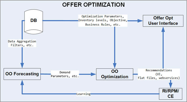
Figure 11-1 shows the conceptual flow of different components in Offer Optimization. ORASE/RI is the core data foundation layer that consumes the retailer data. Offer Optimization Forecasting analyzes historical data to provide the forecasting inputs to the Optimization Algorithm. The Optimization Algorithm obtains inputs such as objectives, budgets, and business rules from the UI, along with optimization parameters from ORASE/RI. The algorithm analyzes the feasible price paths efficiently and generates price recommendations. These recommendations can be viewed in the Offer Optimization UI or can be exported to the price execution systems such as Oracle Retail Price Management (RPM) or Oracle Retail Customer Engagement (CE). In addition, a feedback loop from the price execution systems can help the OO Forecasting component to determine how the offers are performing and adjust the next set of offers based on the sales performance or the response rate. OO supports two kinds of runs, called "ad hoc runs" and "batch runs." Batch runs are scheduled to run automatically at regular intervals (for example, every week). Each batch run, using latest sales data and inventory levels, updates the parameters and budgets and produces the price recommendations. An analyst can review the results and further accept, reject, or override the price recommendations for each item. Once the analyst finishes the review, the item's recommendation status can be changed to Reviewed. A reviewed recommendation is sent to the buyer for approval. If the user with the buyer role likes the recommendations, that user can submit or approve the recommendation. At this point, the recommendation status is changed to Submitted or Approved. This indicates that the price recommendations will be sent to an export interface as well as to a price execution system such as RPM with the respective statuses.

Figure 11-1 Offer Optimization

Description of ''Figure 11-1 Offer Optimization''

An optimization can be carried out at the configured processing (or run) location or the price-zone, merchandise level, and calendar level. The user can configure the optimization to use either the price-zone or a node in the location hierarchy (but not both in the same instance). Once the optimization is complete, the recommendations can be generated at a lower level than the processing level (called recommendation levels for merchandise level and location or price-zone level). The location and merchandise level can be any level in the location hierarchy and merchandise hierarchy, respectively. Alternatively, price-zone can be used to define a set of stores (and/or online locations) and items. An example of a price zone is women's apparel in all university-based stores grouped into one price-zone. The usual levels for the run are Region or Price-zone, Department, and Week, and for the recommendation, the levels are Region or Price-zone and Style/Color or SKU (Style/Color/Size). If Targeted Offers is available, then the recommendations will also be generated at the Customer-Segment level, along with location or price-zone and merchandise level. The Promotions and Markdowns are always at the location or price-zone and merchandise level.

The optimization is set up as follows:

• Optimization is done at the run's merchandise and location setup levels. For example, if the run merchandise and location levels are Department and Region, then each optimization job is at the Department-Region level.

• Inventory is rolled to the desired recommendation level for merchandise. Further, the inventory is aggregated across all the locations to the run's location level.

• Price recommendations are generated at the configured recommendation levels for merchandise, location or price-zone, and calendar level and the customer segment level.

  For example, if the run location level is Price-zone, the run merchandise level is Department, the run calendar level is Week, and the recommendation level for merchandise is Style/Color, then the promotion and markdown recommendations are generated at Price-zone, Style/Color, Week and Price-zone, Style/Color, Week and Customer Segment for Targeted Offers.

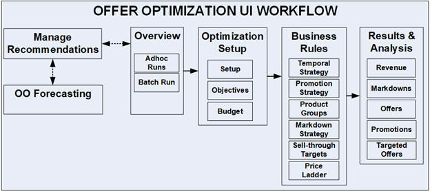
Figure 11-2 shows an overview of the OO UI workflow, which consists of the following:

• Overview. This is the dashboard for the OO runs. In this tab, you can see a list of all existing runs, along with details that describe each run. The list includes runs created by other users, which you can open in read-only mode. You can create a run, copy a run, open a run, or delete a run. The runs overview has three components, Search, Run Status Tiles, and the Table of Runs.

  You can click an existing run or create a new run. Each run is opened in a run tab. The title of the run tab displays "Offer Optimization: <Run ID>". This is the main tab where you can specify the business rules and goals for the run. It provides a series of three stages that you progress through in order to set up, run, and analyze the results of the optimization run.

• Setup. Used to pick a season, location or price zone and department. It is also used to select the objectives and specify the budgets.

• Rules. Used to view or change business rules.

• Results. Used to view results and accept, reject, or override recommendations, and recalculate.

• Forecasting. These screens provide the user with the ability to review the way in which different components of forecast (for example, baseline, seasonality) affect the price recommendation for an item.

• Manage Recommendations. This screen is used to accept, reject, or override and recalculate recommendations. It also allows the user to review, submit, or approve recommendations so that they can be sent to a price execution system. In production, this screen is the starting point and is used most regularly, since the user can send recommendations from batch runs for execution or visit forecasting screens to review how item forecast looks, and finally, decide whether to create a new ad hoc run.

Figure 11-2 Offer Optimization UI Workflow

Description of ''Figure 11-2 Offer Optimization UI Workflow''

The goal of the implementation is to set up and configure an instance to generate optimal price recommendations that satisfy the retailer's business requirements. The implementation configures the application so that the batch runs complete successfully in a timely fashion and produce valid promotions, markdowns, and forecast recommendations that meet the retailer's requirements. The main implementation tasks involve configuring the following:

• The roles and permissions assigned to users.

• The loading of retailer data.

• The configuration parameters.

• The demand parameters, such as seasonality and price effects, that are used to determine optimal promotion, markdown, and targeted recommendations.

• The business rules that determine constraints that the application takes into account during the optimization process.

Security

Offer Optimization supports both data-based and user role-based security. Data security informs the application regarding which merchandise and locations can be accessed by a particular user (for example, the user 'tom' can only access locations within US). The user role restricts or allows which UI actions can be performed by a particular user.

User roles are used to set up application user accounts through Oracle Identity Management (OIM). See Oracle Retail Science Cloud Services Administration Guide for details. Five roles are supported in this application:

• Pricing Administrator

• Pricing Manager

• Pricing Analyst

• Buyer

• Targeted Offer Role

Data Input Requirements

This section provides information about setting up the data that the Offer Optimization application uses to generate optimal price recommendations, including guidelines on the expectations for the data element requested and where it is used. Information about these files can be found in Oracle Retail Insights Cloud Service Suite/Oracle Retail Science Cloud Services Data Interface.

Hierarchy Data

Hierarchies are part of the core data elements that are used in Offer Optimization, in both the forecasting and optimization modules. The four types of hierarchies are Location Hierarchy, Merchandise Hierarchy, Calendar Hierarchy, and Customer Segments Hierarchy. Hierarchy data is required.

• Location Hierarchy. An example of location hierarchy is: CHAIN ' COUNTRY ' REGION ' DISTRICT ' STORE. When the user wants to optimize by location hierarchy, then the run's optimization level must match a node in the location hierarchy. For example, you can run the optimization at the District level. Note that the E-com channel can be defined as part of the location hierarchy.

• Price-zone Hierarchy. OO provides the user with the flexibility to group any set of stores as part of a price-zone and use it as the run setup level for optimization. Here is an example of a price-zone hierarchy: CHAIN ' COUNTRY 'PRICE ZONE'STORE. Note that in OO, a price-zone cannot be defined above country-level since the currencies can be different. Further, the price-zone can be associated with a list of items. Different merchandise in a Department at a particular store can be part of different price zones. For example, women's university apparel in all university-based stores is grouped into one price zone and the women's non-university apparel belongs to another price-zone. If a price-zones are not defined or used, then the UI displays a default value of -1-WORLDWIDE.

  Corresponding interfaces are W_RTL_CLSTR_GRP_DS, W_RTL_CLSTR_GRP_HDR_LC_DS, W_RTL_CLSTR_GRP_PRD_DS, W_RTL_CLSTR_HDR_DS. In C_ODI_PARAM, when the value for CLSTR_PROD_LEVEL is in (DEPT, CLS, SBC) then all MERCH_ID values map to the associated level in W_PROD_CAT_DH. On the other hand, in C_ODI_PARAM, when the value for CLSTR_PROD_LEVEL is in (ITEMLIST), then all MERCH_ID values map to an Item List ID in W_RTL_ITEM_GRP1_D. The later allows the retailer to provide any custom item lists to be mapped to a price zone.

• Merchandise Hierarchy. An example of merchandise hierarchy is as follows: CHAIN ' COMPANY/BANNER 'DIVISION ' DEPARTMENT 'CLASS ' SUBCLASS ' STYLE ' COLOR ' SIZE (SKU). When Offer Optimization is used for fashion apparel, it is expected that the you will provide Style and Color through the relevant interfaces. However, if the retailer deals with merchandise such as electronics, that does not necessarily have style or color, the application will work but some of the UI functionality will not be helpful. For example, Custom Rule has the merchandise selectors Class, Subclass, and Style. If no styles are loaded, then the last selector will not be helpful. Further, in such a situation, the recommendation levels will be at SKU level, as other levels may not be meaningful.

  The STYLE, COLOR and SIZE SKUs are expected to be provided in the W_PRODUCT_DS interface, while the levels between CHAIN and Subclass are provided via W_PROD_CAT_DHS interface. In addition, there must be consistency among the levels provided when using an extended hierarchy. W_PRODUCT_ATTR_DS, is used to indicate the relationship between Style, Style/Color, and Style/Color/Size for an extended hierarchy. If the retailer wants to use an extended merchandise hierarchy, then the retailer must populate this interface.

  Here are the specific fields:

  • PRODUCT_ATTR13_NAME = PROD_NUM for the Style (for example, 0000190086820900)

  • PRODUCT_ATTR14_NAME = PROD_NUM for the Style/Color (for example, 190086834203)

  • PRODUCT_ATTR15_NAME = PROD_NUM for the Style/Color/Size (for example, 1975699). The value of PROD_NUMs is the same as the value in the W_PRODUCT_DS.PROD_NUM interface.

  Here is what this looks like:

  PROD_NUM	PRODUCT_ATTR13_NAME	PRODUCT_ATTR14_NAME	PRODUCT_ATTR15_NAME
  STYLE_PROD_NUM	STYLE_PROD_NUM
  STY/COL_PROD_NUM	STYLE_PROD_NUM	STY/COL_PROD_NUM
  STY/COL/SIZ_PROD_NUM	STYLE_PROD_NUM	STY/COL_PROD_NUM	STY/COL/SIZ_PROD_NUM

  
  

• Calendar Hierarchy. This is one of the core hierarchies. The retailer can specify the calendar depending on their business requirements (for example, fiscal calendar).

• Customer Segments Hierarchy. Offer Optimization supports pricing recommendations at the customer segment level. To use this functionality, the retailer must load customer segments. Note that at this time, the Offer Optimization supports only one customer segment group at a time.

Runs in the Offer Optimization can be set up to run at configured levels for location or price zone, merchandise, calendar, and customer levels.

• Location Level. The run's location processing level is configurable in RSE_CONFIG, and it is denoted as PRO_LOC_HIER_PROCESSING_LVL. For example, a typical level is Region. If the user specifies price-zones, then location level defaults to COUNTRY.

• Merchandise Level. The run's merchandise processing level is configurable in RSE_CONFIG, and it is denoted as PRO_PROD_HIER_PROCESSING_LVL. For example, a typical level is the Class level.

• Calendar Level. The run's calendar processing level is configurable in RSE_CONFIG, and it is denoted as PRO_CAL_HIER_PROCESSING_LVL. For example, a typical level is Week.

• Customer Level. The run's customer processing level is configurable in RSE_CONFIG, and it is denoted as PRO_CUST_HIER_PROCESSING_LVL. For example, a typical level is Segment or Chain (that is, segment-all).

• Setup Level. The run is set up at a level higher than the run's merchandise level. This is configurable in RSE_CONFIG, and it is denoted as PRO_PROD_HIER_RUN_SETUP_LVL. For example, a typical level is Department level.

In this guide, the typical processing levels are generally used as illustration. If necessary, further details will be used to clarify non-typical levels. These levels are also important for the forecasting module since it provides the relevant parameters at the appropriate levels so that it can be consumed by the optimization module.

It is essential that the configuration levels be decided based on the business of the retailer at the time of implementation. These configuration levels dictate how to specify business rules (for example, what is the minimum number of weeks of separation between consecutive markdowns).

Hierarchies are assumed to be set up once for each season and can be revisited whenever it changes. It is expected that the hierarchies do not change from one week to next week within a year (or season). Since hierarchies are core foundational elements any change to hierarchies can be costly and must be planned accordingly. For example, if customer segments are redone, then the parameters must be recalculated. The retailer must plan for such changes as such changes cannot necessarily be completed in the normal weekly batch process or window.

Retail Sales Data

Retail Sales data is a required interface. OO requires you to provide retailer's historical sales data at the desired hierarchy levels. If you want to use the targeted offers, then you must provide the customer-linked transactions sales data. The retailer does not have to provide the data aggregated to the segment-level but must provide the customer ID and customer segment mapping as part of customer segment interface.

Note that the sales returns are handled in the same interface. The returns data identifies the original location where the item was purchased and when it was purchased. This information is useful in returns analysis and in calculating the returns parameters.

When the system is in production, the latest incremental sales data is obtained as part of the batch process.

Promotions

A historical and future planned promotions-related interface is optional. OO allows the user to provide any promotions using the following interface: RSE_PLAN_PROMOTION_STG. This interface provides the retailer with the ability to specify the start and end dates of a promotion event and which merchandise or locations are part of the promotion. This information can help OO in two ways: identify when the promotions have occurred in the past and learn which future planned promotions are similar to the ones in the past. In this interface, the retailer must specify name, when (time), which items, and how deep (for example, for a Father's Day Sale, 20% off all merchandise in Mens division and across all stores).

Warehouse Inventory Allocation

The Warehouse Inventory Allocation interface is optional. The OO user can provide the warehouse to store/online location mapping through this interface (RSE_INV_WHSE_LC_PR_ALLOC_STG). In addition, the user can provide the allocation percentage for each item (that is, how much of warehouse inventory is allocated to the particular store/online location). The user can configure whether to include all components of warehouse inventory in the calculation: warehouse on order, warehouse in transit, warehouse on hand. If the user does not provide the allocation percentages, then OO provides the user with ability to virtually allocate warehouse inventory using an in-built optimization algorithm. The optimization algorithm determines the allocation percentages based on the maximization of revenue across all warehouses.

Competitor Prices

The Competitor Price interfaces, which are optional, are used to provide competitor prices. The two interfaces are W_RTL_COMP_PRICE_IT_LC_DY_FS and W_RTL_COMP_STORE_DS. The retailer can specify the price of an item at multiple competitors/locations and, depending on the configured option, either the minimum or the average of competitor prices is used for the optimization. Competitor prices are used to restrict the price recommendations to a certain percent range of the competitor price. For example, if the retailer wants to match the competitor's promotion of 20 percent off but with some tolerance, then this interface allows the retailer to specify the competitor price through the interface. Tolerance is specified as a global parameter in RSE_CONFIG. Note that in this release, the product can support competitor prices only through an interface.

Product Attributes

The product attributes that are useful in OO forecasting and in particular for targeted offers can be defined through this interface. Raw product attributes (for example, fabric, material, and so on) can be provided through this interface. Make sure the attribute values are as clean as possible. For example, COKE vs. COK vs. COEK must be normalized to COKE so that OO does not interpret them as different attributes.

The retailer must use W_RTL_ITEM_GRP1_DS, since it can support any number of attributes, such as BRAND, and the batch load process picks up the attributes added there automatically. The product attributes that are useful in OO forecasting and in particular for targeted offers can be defined through this interface. Raw product attributes (for example, fabric, material, and so on) can be provided through this interface. Make sure the attribute values are as clean as possible. For example, COKE vs. COK vs. COEK must be normalized to COKE so that OO does not interpret them as different attributes.

If the retailer wishes to load STYLE or COLOR as product attributes, then the W_RTL_ITEM_GRP1_DS interface is used to provide style and color attributes for the different products, using a value in PROD_GRP_TYPE of either STYLE or COLOR. The actual values for the Styles and Colors are provided in columns FLEX_ATTRIB_2_CHAR and FLEX_ATTRIB_4_CHAR using values that represent the ID for the Style (for example, 1234), and a description for the Style (for example, Loose Fit). The columns FLEX_ATTRIB_3_CHAR and FLEX_ATTRIB_10_CHAR contain the appropriate designation for STYLE or COLOR.

OO supports grouping of product attribute values and it is required to load these additional interfaces: RSE_PROD_ATTR_GRP_VALUE_STG and RSE_PROD_ATTR_VALUE_XREF_STG. It is not required to group the attribute values. Consider the following examples:

• Consider Brand attribute with values Adidas, Champion, Nike and Under Armour. Since we are not grouping any attribute values for attribute Brand, each value by itself will be a group.

• Consider the Color attribute. There might be too many variants of the same color and thus it might be meaningful to group the color values. The first interface defines how many groups of colors would be there - for example, Trending, Casual, Professional. The second interfaces maps the actual attribute values to the groups - for example, Trending = {Flame Scarlet, Biscay Green}, Casual={Pink, Green}, Professional={Black, White, Grey}.

• These interfaces can also help with normalization of attribute values. Consider an example when there are a lot of misspellings (for example, COEK vs. COK vs. COEK). The retailer can use this interface to normalize the attribute values and create one group called COKE.

Product Images Data

Product images that are available on a customer-hosted web server can be viewed In OO via the Results screen. The W_RTL_PRODUCT_IMAGE_DS.dat interface contains a column called PRODUCT_IMAGE_ADDR, that can contain the full URL to an image of the product. This URL must be in the following format:

http[s]://servername[:port]/location/filename.extension

For example:

PRODUCT_IMAGE_NAME = imagename.png

PRODUCT_IMAGE_ADDR = http://hostname/url/imagename.png

PRODUCT_IMAGE_DESC= Short description of the image

The OO application running in the cloud does not directly access these images, so there is no need to expose these images outside of the customer's firewall. As long as the user of the OO application has access to the URL while running the OO application, then the user's web browser will be able to resolve the URL and retrieve the images for display when they choose this option. The images must be in a file format that the web browser can display. Since the images shown in the UI are small, these images do not need to be high quality images. The size of the image files will affect the time it takes to render them.

Season

PRO_SEASON_STG is used to define the name of the season with the start and end dates. For example, Halloween Season is used to identify merchandise that sells for Halloween. If the retailer does not have any seasons, then the retailer can define one long season.

Season Periods

PRO_SEASON_PERIOD_STG defines which periods belong to the season and lets users define whether a promotion or a markdown is allowed in a particular period. This interface can include the promotion and markdown calendar information of the retailer.

Season Products

PRO_SEASON_PRODUCT_STG defines which products are associated with a season. This interface indicates which products are to be included in the optimization for recommendations.

Price Ladder

PRO_PRICE_LADDER_STG can be used to supply price ladders. It supports three types of price ladders: Price Point (denoted by type A), Percentage Off Ticket Price (denoted by PT), and Percentage Off Full or Original Price (denoted by PO).

Currency

PRO_COUNTRY_LOCALE_STG can be used to define the currency based on the country. This allows the same instance to support multiple currencies. For example, US locations must generate price recommendations (and price-related metrics) in USD, and Canadian locations must generate price recommendations (and price-related metrics) in CAD. Budgets can be specified in one global currency and optimization runs can be in a different local currency based on PRO_COUNTRY_LOCALE_STG. In which case, budgets are converted based on exchange rates provided in W_EXCH_RATE_GS.

Holidays

RSE_HOLIDAY_STG can be used to define the holidays that are used by the retailer. Major holidays can cause additional traffic visiting the store or the web channel.

Pricing Product Groups

W_RTL_ITEM_GRP1_DS can be used to define the different pricing product groups that are used by the retailer. PRO_OPTIMIZATION_RULES_STG allows the retailer to specify the group types for each of the defined groups. For example, both these interfaces help retailer define which items comprise the group and that this group would need the same markdown discount. Such groups and corresponding constraints are picked up by batch optimization runs.

Budget

W_RTL_PLAN1_PROD1_LC1_T1_FS can be used to specify the budgets for markdowns and/or promotions used by the retailer. A budget can be fed in at the run's merchandise setup-level (for example, Division) or it can be fed in at the run's merchandise processing-level (for example, Department). The interface allows the user to provide separate budgets or a combined budget for promotions and markdowns.

Strategy and Business Rules

PRO_OPTIMIZATION_RULE_STG allows the user to define business rules and associate them with a strategy set. This interface provides the following abilities for the user:

• There will always be a DEFAULT_SET strategy that is reserved to be used by batch runs in production. Other strategy sets are available for the user to do what-if runs.

• It is advised that retailers define all the business rules in the DEFAULT_SET strategy. It is not required that the user define complete set of rules again for a new strategy set. For example, an Aggressive Promotion Strategy set can define rules associated with promotions only. In such a case, the system will try to find the closest rule that is available in DEFAULT_SET when it is not available in the current strategy set.

• In any strategy set, the user can define rules at any merchandise and location levels. Rules will be applied to the merchandise and location that are closest to it. The term "Closest" can be defined as follows: for a given product level, move up the location hierarchy first to find any applicable rule. For example, the user defines Min First Markdown as 10% at Banner- All locations level and 20% for Men's Division-All locations.Then, merchandise in Men's division receives the 20% Min First Markdown rule, and all other merchandise receives the 10% Min First Markdown rule for all locations.

Custom Columns

W_RTL_FLEXFACT_FS can be used to add any custom column to the recommendations in the Manage Recommendation screen. Custom columns are picked up by batch runs at the time of their creation and assigned to the item and location. It supports up to ten numeric columns (for example, last year sales), twenty currency columns (for example, revenue till date), ten text columns (for example, supplier), five percentage columns (for example, sell-through for last four weeks), and five date columns (for example, last markdown date).

Optional Interfaces

The interfaces specified in this section are not required. When the retailer provides the data through the interfaces tagged as 'required', then the system automatically uses the primary interfaces. These are only provided as an alternate source for the same.

• Inventory (RSE_INV_PR_LC_WK_A_STG)

• Price Cost (RSE_PRICOST_PR_LC_WK_STG)

• Optimization Metrics (PRO_SEASON_CURR_OPT_METRIC_STG)

• Model Dates (PRO_MODEL_DATES_STG)

• External Forecast Adjustments (PRO_FCST_EXT_EFFECT_ADJ_STG)

Offer Optimization Integration with Retail Pricing Cloud Service

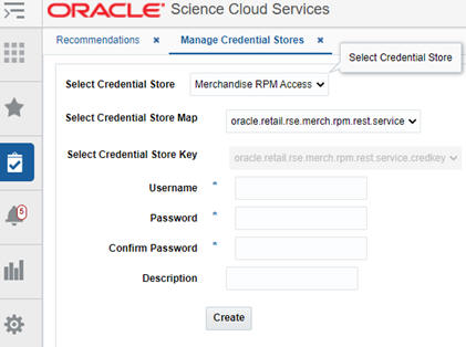
Additional configuration parameters must be set to integrate OO with Retail Pricing Cloud Service. See the list of parameters shown in Table 11-1. In addition, the RPM username and password must be added under the credential store for Merchandise RPM Access. You can modify these values using the UI screen for Control & Tactical Center -> Manage Credential Stores. Control & Tactical Center is available under the task menu.

Setting up the Configuration Parameters for Integration with Retail Pricing Cloud Service

Table 11-1 Configuration Parameters for Integration with Retail Pricing CS

Parameter Name	Parameter Value	Dexcription
PRO_MERCH_RPM_FLG	N	Flag to identify whether to publish markdown recommendations to RPM.
PRO_MERCH_RPM_HOSTNAME		URL host name to publish recommendations to RPM. This must be same as CN name in the certificate.
PRO_MERCH_RPM_CONTEXT_ROOT	RpmRestService/services/private	Context root of the RPM webservice url.
PRO_MERCH_RPM_CLEARANCE_PATH	clearance/induction	Path of the webservice, e.g., clearance/induction.
PRO_MERCH_RPM_PORT	443	Port number to publish recommendations to RPM.
PRO_MERCH_RPM_HTTP_PROXY_HOSTNAME		Proxy host name to publish recommendations to RPM.
PRO_MERCH_RPM_HTTP_PROXY_PORT		HTTP proxy port number to publish recommendations to RPM.
PRO_MERCH_RPM_HTTPS_PROXY_PORT		HTTPS proxy port number to publish recommendations to RPM.
PRO_MERCH_RPM_VERSION	19.0	RPM version to use for publishing customer segment to relate (format 16.0).
PRO_MERCH_RPM_USE_HTTPS	Y	Flag to identify whether to publish markdown recommendations to RPM over HTTPS.
PRO_MERCH_RPM_PROMOTION_PATH	promotion	Path of the RPCS webservice for promotions.

Figure 11-3 Setting up the RPM Access in the Credential Store

Description of ''Figure 11-3 Setting up the RPM Access in the Credential Store''

Configuration and Expected Levels for Interfaces

The expected levels for the interfaces are based on the configuration levels specified for the recommendation and optimization levels. There are five dimensions that are used to define these configurations: Customer (applicable only for targeted offers), Calendar, Merchandise, Location, and Price-zone. The optimization level determines the levels at which optimization is performed. For example, Division and Region (it can also be a price-zone). The recommendation level determines at what levels recommendations must be generated. Typically, these are lower levels of merchandise and location than the optimization levels (for example, Style/Color and Region). Note that the Calendar dimension tells the system at which level recommendations are generated (for example, Weekly vs Daily). The customer dimension tells the system that customer segments are available to generate targeted offers. Promotions and Markdowns are not generated at the customer segment level. If price-zones are not used, then the Price-zone column will be -1. When price-zones are used, then both optimization and recommendation levels will be price-zone. In such a case, both the location configurations, PRO_LOC_HIER_PROCESSING_LVL and PRO_OPT_LOC_REC_LVL, must be set to COUNTRY.

Table 11-2 Configuration: Expected Levels

Data	Configuration Parameters	Customer Segment	Calendar	Merchandise	Location	Price Zone
Optimization Level	Levels at which the optimization process is executed (Units of work)	PRO_CUST_HIER_PROCESSING_LVL	PRO_CAL_HIER_PROCESSING_LVL	PRO_PROD_HIER_PROCESSING_LVL	PRO_LOC_HIER_PROCESSING_LVL	-1 or PZ
Recommendation Level	Level at which the recommendation results are generated	PRO_OPT_CUST_REC_LVL	PRO_OPT_TIME_REC_LVL	PRO_OPT_MERCH_REC_LVL	PRO_OPT_LOC_REC_LVL	-1 or PZ

Depending on the above configuration levels, the interface levels expected are as follows:

Table 11-3 Interfaces: Expected Levels

Data	Interface Name	Notes	Customer	Calendar	Merchandise	Location	Price Zone
Season	PRO_SEASON_STG	Range of time periods (e.g., weeks) for the season. This has to match the calendar hierarchy loaded	N/A	N/A	N/A	N/A	N/A
Season Period	PRO_SEASON_PERIOD_STG	Periods (e.g., weeks) within a season where the PRO_PROD_HIER_PROCESSING_LVL (e.g., CLASS) is active	N/A	PRO_CAL_HIER_PROCESSING_LVL Date range could span multiple calendar units (i.e. Multiple weeks)	PRO_PROD_HIER_PROCESSING_LVL or any hierarchy level higher	PRO_LOC_ HIER_ PROCESSING_ LVL or any other higher hierarchy level	-1 or PZ
Season Product	PRO_SEASON_PRODUCT_STG	Products that must be included in given selling seasons	N/A	PRO_CAL_HIER_PROCESSING_LVL Date range can span multiple calendar units (i.e. Multiple weeks)	PRO_OPT_MERCH_REC_LVL	PRO_LOC_ HIER_ PROCESSING_ LVL	-1 or PZ
Price Ladder	PRO_PRICE_LADDER_STG	Product price ladder	N/A	N/A	PRO_PROD_HIER_PROCESS-ING_LVL or any higher	PRO_LOC_HIER_PROCESSING_LVL	-1 or PZ
Country Locale	PRO_COUNTRY_LOCALE_STG	Defines the specific locale for the location. Provided at the COUNTRY level	N/A	N/A	N/A	PRO_LOC_HIER_PROCESSING_LVL or any hierarchy level higher	N/A
Planned Promotion	RSE_PLAN_PROMOTION_STG	Planned promotion at PRO_PROD_HIER_PROCESSING_LVL (e.g., CLASS)	N/A	PRO_CAL_HIER_PROCESSING_LVL Date range could span multiple calendar units (i.e. Multiple weeks)	PRO_PROD_HIER_PROCESS-ING_LVL	PRO_LOC_ HIER_ PROCESSING_ LVL	-1 or PZ
Holidays	RSE_HOLIDAY_STG	Major holidays	N/A	Date when the holiday is observed	Any level in merchandise hierarchy	Any level in location hierarchy	N/A
Strategy and Business Rules	PRO_OPTIMIZATION_RULE_STG	Business rules and associated strategies	N/A	N/A	Any level in merchandise hierarchy	Any level in location hierarchy	N/A

Table 11-4 Expected Levels for Optional* Interfaces

Data	Interface Name	Notes	Customer	Calendar	Merchandise	Location	Price Zone
Model Start Dates	PRO_MODEL_DATES_STG	Model start and end date for each product	N/A	PRO_CAL_HIER_PROCESSING_LVL	PRO_OPT_MERCH_REC_LVL	N/A	-1 or PZ
Optimization Metrics	PRO_SEASON_CURR_OPT_METRIC_STG	Updates (e.g., weekly) for mkdn and promo price, mkdn and promo count and mkdn and periods when item was promoted	N/A	PRO_CAL_HIER_PROCESSING_LVL	SKU level (Style/Color/Size)	Store	N/A
Inventory	RSE_INV_PR_LC_WK_A_STG	Inventory available at the start of the period (e.g., week). Inventory is aggregated to the PRO_LOC_HIER_PROCESSING_LVL (e.g., Price Zone)	N/A	Week	SKU level (Style/Color/Size)	Store	N/A
Price Cost	RSE_PRICOST_PR_LC_WK_STG	Price cost for the time period (e.g., week)	N/A	Week	SKU level (Style/Color/Size)	Store	N/A

Offer Optimization Forecasting

Offer optimization forecasting has two modules, parameter estimation and demand forecasting. Parameter estimation uses the historical data to determine the seasonality, markdown elasticity, promotion elasticity, and promotion lift (or holiday lift) values. Demand forecasting leverages the parameters estimated from historical data and in-season sales data (the base demand is re-estimated on a regular basis as part of batch process) to determine the demand and generate the forecast.

Offer optimization forecasting supports the following features:

• Separate elasticity values for promotions and markdowns

• Customer segment level parameter values for seasonality, elasticity, and traffic lift for promotion and holidays

• The weather effects from historical data period can be incorporated into the estimation of parameters to remove the bias introduces by weather on forecasted sales.

• The ability to execute the following analysis:

  • Day of the week and time of the day profiles

  • Returns analysis

For both parameter estimation and demand forecasting stages, you can set up runs and configure various settings using the Manage Forecast Configurations functionality under Strategy & Policy Management. Based on the configuration settings, a batch job is used to initially estimate the parameters and then update them at specified intervals to reflect the latest sales trends. Similarly, a weekly batch job is used to generate demand forecasts every week after the weekly data has been updated.

Parameter Estimation

Parameter estimation consists of the following stages. Each stage has a series of configurable parameters and the corresponding default values. Modify the default values appropriately for each retailer. You can modify these settings using the Manage Forecast Configurations functionality under Strategy & Policy Management.

Overview of the Parameter Estimation Stages

The following sections describe the details of the settings in each stage..

1. Data preparation. Defines the levels to which data is aggregated on merchandise, location, customer segment, and time dimensions and the duration of the data used for parameter estimation.

2. Preprocessing. Filters the historical data and makes the first determination of item eligibility.

3. Elasticity. Determines the price elasticity for markdowns and promotions.

4. Seasonality. Estimates seasonality trends and identifies partitions with reliable seasonality.

5. Promotion lift. Estimates the traffic lift during promotion and holiday events. Corrects the seasonality curves to remove the traffic lift from promotion and holiday events.

6. Output. Generates parameter files in the format required by demand forecasting and offer optimization.

The parameter estimation stage generates markdown elasticity, promotion elasticity, seasonality and promotion lift values. Together they are referred to as demand parameters.

Parameter estimation requires at least 20 months of data. These requirements exist for the following reasons.

• The data from the beginning 4-6 weeks of the historical period must be removed from the data analysis so that the items that have truly started selling after the beginning of historical data period can be identified.

• The full life cycle data is required for all fashion/seasonal merchandise introduced during a fiscal year in order to estimate the seasonality curve for merchandise starting in every fiscal month. The least amount of data required is one year plus the typical season length of the merchandise.

Data Preparation

The data preparation stage defines the aggregation levels on merchandise, location, customer-segment, calendar dimensions, and duration of the data used for parameter estimation.

In addition to the above, configuration of the hierarchy level at which promotion data is processed is completed here.

Data Aggregation

Sales data, inventory data, and returns data are aggregated on the following dimensions: Merchandise, Location, Price Zone (if available), Customer Segment (if available), and Calendar. The hierarchy type ID corresponding to each dimension is configured using the following parameters in the RSE_CONFIG table. Use the Manage System Configurations functionality to set the appropriate ID for each dimension.

The level of aggregation for each dimension can be configured while setting up the forecast run types in Manage Forecast Configurations. In addition, while creating a run type, the user can indicate whether Price Zone and Customer Segment should be used as additional dimensions in the aggregation process.

• Merchandise (PMO_PROD_HIER_TYPE). Multiple hierarchy types are available for Merchandise, Product, and Extended Product hierarchies. Choose the ID corresponding to the appropriate product hierarchy. Typically, data is aggregated to Style/ Style-Color level on the merchandise hierarchy. Select the appropriate merchandise level when setting up the forecast run type in Mange Forecast Configurations.

• Location (PMO_LOC_HIER_TYPE). Multiple hierarchy types are available for location, for example, Location Hierarchy and Trade Area Hierarchy. Choose the ID corresponding to the appropriate location hierarchy. Typically, data is aggregated to Store Cluster/Price Zone level. Choose the appropriate level. Select the appropriate location level when setting up the forecast run type in Manage Forecast Configurations.

• Customer Segment (PMO_CUST_SEG_HIER_TYPE). Choose the hierarchy type ID associated with the customer segment. By default, customer segment data is aggregated at two levels, by individual customer segments and Segment-All, which includes all the segments. The user does not have the option to select the aggregation level by customer segment.

• Calendar (PMO_FISCAL_CAL_HIER_TYPE). Choose the hierarchy type ID associated with the Calendar hierarchy.

Table 11-5 Data Aggregation

Setting Name and Description	Default Value	Range of Values
Merchandise Hierarchy Type ID: ID corresponding to the merchandise hierarchy used for aggregation of sales, inventory, and returns data.PMO_PROD_HIER_TYPE	3	1 - 15
Location Hierarchy Type ID: ID corresponding to the location hierarchy used for aggregation of sales, inventory, and returns data.PMO_LOC_HIER_TYPE	2	1 - 15
Customer Segment Hierarchy Type ID: ID corresponding to the customer segment hierarchy used for aggregation of sales, inventory, and returns data.PMO_CUST_SEG_HIER_TYPE	4	1 - 15
Calendar Hierarchy Type ID: ID corresponding to the calendar used for aggregation of sales, inventory, and returns data.PMO_FISCAL_CAL_HIER_TYPE	11	1 - 15
Merchandise Level: Level in the merchandise hierarchy at which data is aggregated for sales, inventory, and returns. Typically, data is aggregated to STYLE-COLOR. Choose the appropriate level when setting up the forecast run type in Manage Forecast Configurations.	8	1 - 9
Location Level: Level in the location hierarchy at which data is aggregated for sales, inventory, and returns. Typically, data is aggregated to STORE CLUSTER. Choose the appropriate level when setting up the forecast run type in Manage Forecast Configurations.	5	1 - 6
Calendar Level: Level in the calendar hierarchy at which data is aggregated for sales, inventory, and returns. Choose the appropriate level when setting up the forecast run type in Manage Forecast Configurations.	4	1 - 5
Keep temporary tables: Turn this setting on to retain the intermediate tables generated during the parameter estimation process. PMO_KEEP_TEMP_TABLES	N	Y/N

Promotion Data Processing Level

Promotions data can be present at various levels in the merchandise and location hierarchy. Choose the level at which promotions are defined for estimating traffic lift values. For estimating traffic lifts, we consider major events which drive significant traffic across the chain. For example: there events are defined at country-banner level.

Table 11-6 Hierarchy Levels Selection

Setting Name and Description	Default Value	Range of Values
Promotion processing level Merchandise. Choose the ID corresponding to the merchandise level at which traffic driving promotions are defined. Usually this is Company/Banner if there are multiple banners within the company. PMO_MIN_LOC_HIER_PROCESSING_LVL	2	1 - 9
Promotion processing level - Location: Choose the ID corresponding to the location level at which traffic driving promotions are defined. Usually this is Chain/Country level. PMO_MIN_PROD_HIER_PROCESSING_LVL	2	1 - 6

Data Validation

Once the data preparation stage is complete, prepare data validation report and review it with the customer to confirm the data loaded matches with their expectations. Include the following in the data validation report.

• Summary of merchandise, location, customer segment, calendar hierarchies

• Sales units and amount by year at Chain and Division levels

• Summary metrics by Department-Price zone

• Sales, Inventory and Product count trends by Fiscal week and Fiscal year at Country-Banner level

• For the following data fields Ticket price, sales price, Item cost, Sales units, Sales amount, Inventory

  • Search for negative and null values

  • Significant percent of records with either negative or null values. Flag for review with customer.

Validating data with the customer is key to identifying potential data related problems early on. Investigate any potential data issues and work with the customer to resolve them. This ensures that the following stages are using the appropriate data.

Preprocessing

The Preprocessing stage filters the historical data to produce a subset of data that produces reliable demand parameters. The Preprocessing stage applies filters at the partition and week level. It performs the initial pruning of bad activity data. It does the first stage of determining eligibility and calculates certain values that can later be used in the calculation of elasticity and seasonality parameters. You can modify the configuration settings for the preprocessing stage using the Manage Forecast Configurations functionality under Strategy & Policy Management.

Data Filters Week Level

Table 11-7 shows the various week level filters used in the Preprocessing stage. These filters are used to remove individual weekly records of data that do not meet the requirement defined as specified for each filter.

Table 11-7 Data Filters Week Level

Filter Name and Description	Default Value	Range of Values
Store count greater than 0. Used to filter activities with null or zero store count. IWF_STORE_GTR_ZERO	N	Y/N
SKU store count greater than 0. Used to filter activities with null or zero sku store count. IWF_SKU_STORE_GTR_ZERO	N	N/Y
Inventory data present. Used to indicate that the inventory data is available and reliable. If inventory data is available and reliable, then Preprocessing will use inventory data for filtering and other calculations. If inventory data is not available or unreliable, then it is ignored. IWF_INV_DATA_PRESENT	Y	N/Y
Sales unit threshold. Used to filter sales data records with sales units below threshold values. IWF_SALES_UNIT_THRESHOLD	1	Greater than or equal to 1.
Inventory threshold. Used to filter sales data records with inventory units below threshold values. IWF_INV_THRESHOLD	1	Greater than or equal to 0.
Use store count for Inventory threshold. Defines the criteria used for inventory threshold. Setting to Y will use Store count with inventory as inventory threshold criteria instead of actual inventory value. IWF_SKU_STORE_COUNT	N	Y/N
Threshold combination. Use AND/OR combination for Sales unit threshold and Inventory threshold.IWF_FILTER_COMBO	AND	AND/OR
Life cycle sell thru %. The item start and end dates are calculated using percentage sell through. The start date is the date when Life cycle sell through % (Start) is reached. The end date is the date when Life cycle sell through % (End) is reached. Life cycle sell through % (Start) is expressed relative to 0% so entering 2 means that the start date is when 2% of total sales has been achieved. Life cycle sell through % (End) is expressed relative to 100% so entering 2 means that the end date is when (100-2)% i.e., 98%, of total sales has been achieved. IWF_LOW_LCYCLE_SELL_PCT and IWF_HIGH_LCYCLE_SELL_PCT	Start: 2.0 End: 2.0	Start: greater than or equal to 0; less than or equal to 50. End: greater than or equal to 0; less than or equal to 50.
Relative price. Relative price thresholds are used to filter out item weeks with a ratio of sales price to maximum ticket price that fall outside the specified range for the start date and the end date. IWF_LOW_RELATIVE_PRICE and IWF_HIGH_RELATIVE_PRICE	Start: 0.2 End: 1.0	Start: greater than 0. End: greater than the start value.

Partition Filters

These filters are used to exclude all the weekly records from a Merchandise-Location-Customer segment partition at the aggregation level, for partitions with values that do not meet the requirement specified for each filter, as described below.

Table 11-8 Partition Filters

Filter Name and Description	Default Value	Range of Values
Minimum number of eligible weeks. Aa certain number of weeks are necessary in order to determine item eligibility. IF_MIN_ELIGIBLE_WEEKS	6	Greater than 0.
Minimum season (weeks). A certain season length (the number of weeks between the first and last activity) is required in order to determine item eligibility. IF_MIN_SEASON_WEEKS	6	Greater than 0.
Minimum sales units. The total number of units sold must be at least this value. IF_MIN_SALES_UNITS	10	Greater than 0.
Fraction of eligible weeks. The percentage of eligible weeks, expressed as a fraction of the season length. The season length is the number of weeks between the start and end dates. (See Life cycle sell thru % above.) IF_FRACTION_ELIGIBLE_WEEK	0.6	Greater than 0.0; less than or equal to 1.0.

Elasticity

The Elasticity stage determines the promotion and markdown elasticity values at the selected levels in the merchandise and location hierarchy. For a given merchandise and location hierarchy level, this stage also determines the elasticity value by customer segment. You can modify the configuration settings for the elasticity stage using the Manage Forecast Configurations functionality under Strategy & Policy Management.

In this stage, parameters must be set for

• Additional data filtering to reduce the noise in the elasticity estimation

• Merchandise and location hierarchy levels for which parameters are estimated

• Identifying markdowns weeks

• Identifying promotion weeks

• Reliability thresholds for elasticity estimation

• Transformation of elasticity values

Data Filters Weekly

Additional data filters are applied during the estimation of elasticity. These filters are used to reduce the noise from very deep price cuts or price cuts towards the end of life. An option is also available to the limit the data used for elasticity estimation.

Table 11-9 Data Filters Weekly

Filter Name and Description	Default Value	Range of Values
Relative price. Used to filter out item-weeks with a ratio of sales price to maximum ticket price that falls outside the specified range. WDF_RELPRICE_LOW and WDF_RELPRICE_HIGH	Low: 0.2 High: 1.0	Low > = 0; High > low value
Relative inventory. The upper and lower bounds for the value for inventory relative to maximum inventory. WDF_PCTSALES_LOW and WDF_PCTSALES_HIGH	Low: 0.2 High: 1.0	Greater than or equal to 0. Low > = 0 High > low value
Range filter. Used to eliminate unreliable data using start date and end date for the period. Both the start date and the end date are Null by default. A Null value means that the field is not used in the filter. One or both of the fields can have a value of Null. If both of the fields are Null, then the data is not filtered. WDF_RANGEFILTER_MINCALWK and WDF_RANGEFILTER_MAXCALWK	Start date: Null End date: Null	-

Hierarchy Levels Selection

Select the merchandise and location levels for which parameter estimation should calculate demand parameters. Parameter estimation calculates demand parameters for the partitions of the levels that are the cross-products of all the levels you select. The highest level is set based on PMO_MIN_LOC_HIER_PROCESSING_LVL (typically, Banner) and PMO_MIN_PROD_HIER_PROCESSING_LVL (typically, Department). The lowest level is set based on the aggregation levels that the user selects while creating the forecast run types. In Manage Forecast Configurations, the user can select from the list of levels that are between the highest and lowest levels.

Markdowns

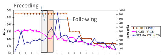
The parameters described below are used to identify markdowns in the aggregated weekly sales data. During a markdown window, the application is interested in a drop in prices from the preceding window to the following window. During a promotion, the application is looking for similar prices during the preceding and following window but a drop in prices during the promotion window. Similar parameters are used to identify Promotions as well.

Figure 11-4 Markdown Window

Description of ''Figure 11-4 Markdown Window''

Time window defines the weeks before and after the markdown. The preceding weeks value is the number of weeks before the markdown occurred. The following weeks value is the number of weeks after the markdown and includes the week of the markdown. A week is a calendar week. A time window that satisfies all the markdown parameter settings is classified as a markdown window.

Minimum eligible weeks is the minimum of the actual number of weeks in the Time Window that have data. The Time Window is in calendar weeks, and not every calendar week actually has sales data. So the actual number of weeks with data that are within the Time Window can actually be smaller than the Time Window.

Maximum deviation is the deviation of the sales price in the weeks before and after the markdown. Provides stability on the variance.

Min Markdown depth is the drop in average sales price from preceding weeks to the following weeks is higher than this threshold value. Markdown depth = 1- (Avg Price following weeks/Avg Price preceding weeks). In other words, this parameter controls how much of a price decrease is required in order for the price decrease to count as a markdown.

Table 11-10 Markdown Parameters

Name and Description	Default Value	Range of Values
Time Window MKDN_TIMEWINDOW_PRECEEDING and MKDN_TIMEWINDOW_FOLLOWING	Preceding: 2 Following: 2	1–3 1–3
Eligible Weeks MKDN_ELIGWKS_PREC and MKDN_ELIGWKS_FOLL	Preceding: 2 Following: 2	1–3 1–3
Maximum Deviation MKDN_MAXDVT_PRECEEDING and MKDN_MAXDVT_FOLLOWING	Preceding: 0.1 Following: 0.1	0–1 0–1
Min Markdown Depth MKDN_MINMKDN_DEPTH	0.1	0–1
Use Ticket Price: Both Ticket price and sales price values from the preceding and following weeks satisfy min markdown depth criteria. USE_TICKET_PRICE	N	Y/N

Promotion One Week

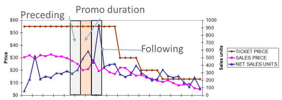
For identifying promotions, a few additional parameters are defined below in addition to Time window, Eligible weeks, and maximum deviation, which are defined above.

Figure 11-5 Promotion Window

Description of ''Figure 11-5 Promotion Window''

Min Promotion depth is the drop in average sales price during the week of promotion compared to preceding/following weeks. In other words, this parameter controls how much of a price decrease is required in order for the price decrease to count as a promotion.Time window defines the weeks before promotion, during promotions, and after the promotion. The preceding weeks value is the number of weeks before the markdown occurred. The following weeks value is the number of weeks after the markdown and includes the week of the markdown. A week is a calendar week. Time window that satisfies all the promotion parameter settings is classified as a promotion window.Promotion depth = 1- (Avg. Price during promotion weeks/ Avg. price during preceding and following weeks). Time Window - Promo duration: Duration of the promotion event, this is set to 1 for 1-week promotion. Max deviation - Preceding/Following: Avg. price deviation across preceding and following weeks must be less than this threshold. This ensures that the sales price is similar in the weeks before and after the promotion.

Table 11-11 Promotion Parameters

Name and Description	Default Value	Range of Values
Time Window PRWK1_TIMEWINDOW_PRECEEDING, PRWK1_TIMEWINDOW_FOLLOWING and PRWK1_TIMEWINDOW_PROMOWEEKS	Preceding: 1 Following: 1 Promo Duration: 1	1–3 1–3 1
Eligible Weeks PRWK1_ELIGWKS_PREC and PRWK1_ELIGWKS_FOLL	Preceding: 1 Following: 1	1–3 1–3
Maximum Deviation PRWK1_MAXDVT_PRECEEDING, PRWK1_MAXDVT_FOLLOWING and PRWK1_MAXDVT_PRECFOLLOW	Preceding: 0.1 Following: 0.1 Preceding/Following: 0.1	0–1 0–1 0–1
Min Promotion Depth PRWK1_MINPROMO_DEPTH	0.1	0–1

Promotion Two Week

Promotion duration parameter is set to 2 for identifying two week promotions. Promotion parameters for one week and two week promotions can be set to different values.

Table 11-12 Promotion Two Weeks

Name and Description	Default Value	Range of Values
Time Window PRWK2_TIMEWINDOW_PRECEEDING, PRWK2_TIMEWINDOW_FOLLOWING and PRWK2_TIMEWINDOW_PROMOWEEKS	Preceding: 1 Following: 1 Promo Duration: 2	1–3 1–3 2
Eligible Weeks PRWK2_ELIGWKS_PREC and PRWK2_ELIGWKS_FOLL	Preceding: 1 Following: 1	1–3 1–3
Maximum Deviation PRWK2_MAXDVT_PRECEEDING, PRWK2_MAXDVT_FOLLOWING and PRWK2_MAXDVT_PRECFOLLOW	Preceding: 0.1 Following: 0.1 Preceding/Following: 0.1	0–1 0–1 0–1
Min Promotion Depth PRWK2_MINPROMO_DEPTH	0.1	0–1

Reliability Settings

Determine the partitions with reliable elasticity values.

Table 11-13 Reliability Settings

Name and Description	Default Value	Range of Values
Outlier threshold. Percentile threshold for removing outlier data points from elasticity estimation. Eg., Threshold is set to X%, Top X Percentile and Bottom X percentile sales ratio and price ratio data points are excluded from elasticity estimation. RS_OUTLIER_THRESHOLD	0.05	0–0.05
Eligible items threshold - Elasticity RS_ELIGIBLEITEMS_THRESHOLD	25	Greater than 1.
Std. Error threshold RS_STDERROR_THRESHOLD	0.3	0–1

Transformation

Transform the elasticity values obtained after the pruning based on reliability to cap the very low or very high elasticity values. The transformation settings also enable the user to shift the elasticity values to a desired range.

Table 11-14 Transformation

Name and Description	Default Value	Range of Values
Transform Percentile - Low TRANSPERCENTILE_LOW	0.1	0–1
Transform Percentile - High TRANSPERCENTILE_HIGH	0.9	0–1
Elasticity range - Min: Select a value closer to the transform percentile - Low and higher than 1.2 ELASTICITYRANGE_MIN	1.3	Greater than 1.
Elasticity range - Max: Select a value closer to the transform percentile - high. ELASTICITYRANGE_MAX	2.8	Greater than elasticity range–min.

Seasonality

The Seasonality stage determines the seasonality values at the selected levels in the merchandise and location hierarchy. For a given merchandise and location hierarchy level, this stage also determines the seasonality value by customer segment. You can modify the configuration settings for the seasonality stage using the Manage Forecast Configuration functionality under Strategy & Policy Management.

In this stage, parameters must be set for

• Seasonality curve set up

• Reliability filters

Seasonality Curve Setup

The Seasonality Curve Setup stage determines the season codes used for building seasonality curves, length of the seasonality curve, item count threshold, padding curve weight, and seasonality coverage of the final curves.

Season codes create additional partitioning in the dataset by introducing a time dimension. This stage can be used to partition seasonality curves by fiscal start month, fiscal start week, for example, Partition the Class-Store cluster-Customer segment data based on the merchandise time of introduction. Group merchandise based on the fiscal month of the start date. This ensures items starting in the same month receive the same season code. Weekly curves are useful for modeling short life cycle merchandise, while monthly curves are useful for medium to long life cycle curves.

Length of the seasonality curve: Seasonality curves are generated for 52 weeks. They can also be generated for longer duration if the merchandise life cycle length is longer. This also increases the duration of historical data required to prepare the seasonality curves.

Actual sales for a given merchandise-location-customer segment-Start month can be present for less than 52 weeks. To generate a curve for the entire 52 weeks duration, a padding curve is used.

Padding curve: The padding seasonality curve is determined by creating a basic curve for the highest merchandise/location partition. The final seasonality curve is calculated as weight * padding curve + (1 - weight) * seasonality curve.

Table 11-15 Seasonality Curve Setup

Name and Description	Default Value	Range of Values
Curve Type. Determines the duration of time partition based on fiscal week or fiscal month. CURVE_TYPE	Monthly	Monthly or Weekly
Basic Curve. Basic curves are generated by ignoring the partitioning on time dimension for a given merchandise-location-customer segment partition. BASIC_CURVE	Y	True or FalseY/N
Seasonality curve length. Determines the length of the final seasonality curves for regular (non-basic) season codes. The length from the start determines how many weeks after the start date are in the curve. SEASON_CURVE_LENGTH	52	Greater than or equal to 6.
Eligible items threshold. The minimum number of items that a Merchandise Hierarchy/Location Hierarchy/Customer Segment/Season Code partition must contain so that Raw-AP can produce a seasonality curve for the partition. ELIGIBLE_ITEM_THRESHOLD	5	Greater than or equal to 1.
Padding curve weight. The value used in determining the final seasonality curve. PADDING_CURVE_WEIGHT	0.4	Greater than 0.0; less than 1.0.
Basic curve start week. First week of the basic curve. This is represented as number of weeks from the most recent week with data. Should be greater than 52 and less than number of weeks of historical data.	57	52 - 80
Seasonality Coverage. First Fiscal year SEASON_COVERAGE_FIRST_FY	Latest fiscal year with historical data	Greater than or equal to 2020
Seasonality coverage. Last fiscal year SEASON_COVERAGE_LAST_FY	Latest fiscal year with historical data + 2.	Greater than or equal to 2020.

Reliability Filters

The filters in this stage are used to identify reliable seasonality curves based on the number of items in the partition, average sales volume, and season length threshold.

Table 11-16 Reliability Filters

Name and Description	Default Value	Range of Values
Keep top level curves. All the highest level curves are kept, regardless of threshold values. KEEP_TOP_LEVEL_CURVES	Y	Y/N
Prune curves with missing dates. Pruning of basic curves with missing dates is permitted. PRUNE_CURVES_MISSING_DATES	Y	Y/N
Eligible items threshold. Partitions with fewer numbers of eligible items than the threshold value are removed. Eligibility is defined during preprocessing.	5	Greater than or equal to 0.0.
Average weekly sales threshold. Partitions with average weekly sales below the threshold are removed. Weekly sales are the sum of all sales for all activities for a given week. AVG_WK_SALES_THRESHOLD	25	Greater than or equal to o.
Raw seasonality length threshold. Curves can be discarded when the number of weeks from the first non-zero seasonality value to the last non-zero seasonality value is less than the threshold. In the seasonality stage, it is possible that many seasonality values of zero have been added to the curves. Note that basic season codes have a length of 53, so picking a value greater than 53 will prune out any basic season codes. Seasonality curves before padding are referred to as raw seasonality curves. RAW_SEASONALITY_LEN_THRESHOLD	10	Greater than or equal to 0.

Promotion

The promotion stage determines the traffic lift value associated with promotions and holiday events at the selected levels in the merchandise and location hierarchy. For a given merchandise and location hierarchy level, this stage also determines the promotion lift value by customer segment. A list of holidays and promotions, along with event start date and end date, is sent as a data feed.

In this stage, parameters must be set for determining the baseline to be used for estimation of lift values, Outlier threshold, min lift value. and max lift value. You can modify the configuration settings for the promotion stage using the Manage Forecast Configurations functionality under Strategy & Policy Management.

Table 11-17 Promotion

Name and Description	Default Value	Range of Values
Baseline. The baseline type determines how to smooth the seasonality curve. If you select the linear option, parameter estimation looks at event effective start date and event effective end date and draws a straight line between them. Effective start date is the weekend prior to the event start date and effective end date is the second weekend after the event end date. PROM_LIFT_BASELINE_TYPE	Linear	Linear, Min, or Max.
Outlier percentile.Very high lift values are flagged. PROM_LIFT_OUTLIER_PERCENTILE	0.05	0–1
Lift value -High. Lift values flagged as outliers are capped to outlier percentile lift value. PROM_LIFT_HIGH	Y	Y/N
Lift value-min. Sets the threshold for min lift value. Any promotions with lift value lower than this threshold are not assigned any lift value. PROM_LIFT_MIN_VALUE	1.05	Greater than or equal to 1.

Output and Review of Parameters

The Propagation and Parameter Export to Target stages do not have separate settings. The Propagation stage populates the seasonality curves for all the years from the Seasonality coverage first fiscal year to the Seasonality coverage last fiscal year.

The Parameter Export to Target stage populates the parameters at the lowest level of estimation selected in the appropriate output tables. Offer Optimization typically expects the parameters at the lowest level of estimation. For example, Offer Optimization expects the demand parameters at Class-Store cluster level. Use escalation to fill in the parameters missing at Class-Store level. The Output stage escalates on location hierarchy first and then on merchandise hierarchy.

Run the parameter estimation by starting the batch process during the implementation phase. Details on the batch processing are covered in "Batch Processing". PMO_LOG_TBL can be used to track the progress of the run. Once the parameter estimation is complete, review the parameter values using the Innovation Workbench. Perform the following checks after each stage in the parameter estimation is complete.

Elasticity (pmo_elasticity_parameters)

• Histogram of elasticity values, promotion vs markdown: Distribution of elasticity values follows the expected trend. Typically follow a normal distribution around the median elasticity value.

• Elasticity escalation: Percentage of partitions receiving elasticity values from higher level.

Seasonality (pmo_seasonality_parameters; pmo_seasonality_curve_tbl)

• Review number of partitions impacted by reliability filters:

• Visually check the top level seasonality curves

• Seasonality escalation: Percentage of partitions receiving elasticity values from higher levels.

Promotion lift (pmo_promtion_lift)

• Plot histogram of promotion lift values by event and compare across segments.

Day Level and Returns Metrics

This section covers the settings used for determining day of the week profiles, time of the day profiles, return rate, and average time to return.

Day of the Week Profiles

Day of the week profiles determine the relative sales strength across various days in a given week. These profiles are used to spread the forecasted demand to the day level. In order to capture the variation across merchandise, location, segment, and calendar dimension, the configuration on each of the four dimensions is supported. In the current version, you can choose two configurable levels for estimating day of the week profiles. Level 1 corresponds to the estimation level at which profiles are calculated, and Level 2 profiles correspond to the escalated profiles. They are only used when profiles are not available at the estimation level.

Table 11-18 Day of the Week Profiles

Name and Description	Default Value	Range of Values
Merchandise level. ID corresponding to the merchandise level at which day of the week profiles are calculated. Usually at DEPARTMENT or higher. RSE_PMO_DLYPROF_MH_LVL_SQC1	4	1 - 9
Location level. ID corresponding to the location level at which day of the week profiles are calculated. Usually STORE CLUSTER or higher. RSE_PMO_DLYPROF_LH_LVL_SQC1	4	1 - 6
Merchandise level. Merchandise level - Escalated: ID corresponding to the higher merchandise level at which day of the week profiles are calculated. Usually at Division or higher. RSE_PMO_DLYPROF_MH_LVL_SQC2	3	1 - 3
Location level. Location level - Escalated: ID corresponding to the higher location level at which day of the week profiles are calculated. Usually Region or higher. RSE_PMO_DLYPROF_LH_LVL_SQC2	3	1 - 3
Min week. Calendar hierarchy ID corresponding to the oldest week used for day of the week profile calculation. PMO_DLYPROF_MIN_WK	User determined
Max Week. Calendar hierarchy id corresponding to the latest week used for day of the week profile calculation.PMO_DLYPROF_MAX_WK	User determined
Week count threshold. Partitions with data for less than the week count threshold are excluded from day of the week profile calculation. PMO_DLYPROF_WK_CNT_THLD	2	> 1
Sales threshold. Total sales from the merchandise, location, segment and calendar partition must be higher than this threshold value for the partition to be eligible for estimation of day of the week profile. PMO_DLYPROF_TOT_SLS_THLD	1000	Greater than 100.
Output level - Merchandise. Day of the week profiles are generated at this merchandise level for export. Any missing levels are filled using the higher level profiles.	4	1 - 9
Output level - Location. Merchandise: Day of the week profiles are generated at this location level for export. Any missing levels are filled using the higher level profiles.	4	1 - 6

Returns Metrics

For returns parameter estimation, the data is divided into two parts, one for building the model and the other for testing the model. Usually, one full year is used to build the model, and at least 13 weeks are used for testing the model. The most recent data corresponding to the build and test durations is used for returns modeling from the available data. Returns are modeled at various locations in the merchandise hierarchy, typically, Class, Department, and Division. For each of the merchandise levels, modeling is done for both customer segment and segment all levels on the customer segment dimension and at the data aggregation level on the location dimension. After applying the reliability filters, the missing parameters at the lowest merchandise level - location: data aggregation level - customer segment level are filled by escalation.

The return rate is estimated at the data aggregation level for the Merchandise-Location-Customer Segment level every week. This information, along with the returns parameters and sales forecast, is used to generate the returns forecast.

Table 11-19 Returns Metrics

Name and Description	Default Value	Range of Values
Merchandise level 1. The top most merchandise level used for returns parameters. Typically Division or Banner. Choose the merchandise hierarchy ID corresponding to this level. PMO_RETURN_PART_MH_LVL1	2	1 - 6
Merchandise level 2. The intermediate merchandise level used for returns parameters. Typically Department. Choose the merchandise hierarchy ID corresponding to this level.PMO_RETURN_PART_MH_LVL2	4	1 - 6
Customer segment level 1 Merchandise level 2. The lowest merchandise level used for returns parameters. Typically Class. Choose the merchandise hierarchy ID corresponding to this level.PMO_RETURN_PART_MH_LVL3	5	1 - 6
Duration of data for Build. Number of weeks of data to be used for building the model. PMO_RETURN_BUILD_MODEL_WKS	52	52 - 80
Duration of data for Test: Number of weeks of data to be used for testing the model. Most recent weeks are used for testing the model. PMO_RETURN_TEST_MODEL_WKS	13	13 - 26
Sales threshold. Merchandise-Location-Customer segment partitions with total sales lower than the threshold are excluded from returns parameter estimation. PMO_RETURN_LOW_SALES_THRESHOLD	10	> 10
Model fit threshold. Merchandise-Location-Customer segment partitions with adjusted r square value lower than the threshold are pruned. This eliminates partitions where the model fit is poor. PMO_RETURN_RELIABLE_ADJST_R_SQR_THSLD	0.5	> 0.3
Data sufficiency threshold. Row count: Merchandise-Location-Customer segment partitions: Total with data less than the row count threshold are excluded from returns parameter estimation. PMO_RETURN_RELIABLE_ROW_COUNT_THSLD	500	>100

Demand Forecasting

The following multiplicative demand model is used as follows:

Demand = Base demand* Seasonality *Price effect* Promotion Traffic Lift*Store count* Other Effects

Base demand is updated in season every week at the Optimization recommendation level, for example, Style Color-Store cluster-Customer segment level. Demand forecasting leverages the parameters estimated from historical data and in-season sales data to generate a demand forecast. Elasticity for determining price effect is assigned using merchandise and location hierarchy. For assigning seasonality curve and promotion lift, the start date is required to determine the right partition on time dimension in addition to merchandise and location hierarchy. Demand forecasting set up involves configuration for start date and demand strategy.

Demand forecasting stage leverages the parameters estimated from historical data and in-season sales data to generate a demand forecast. Demand forecast values along with historical parameters are sent to Offer Optimization for generating optimal price recommendations and targeted offers.

In this stage, the following parameters must be set by the user to determine the model start date, season code and demand model settings. For all the parameters prefixed with RSE, you can modify the values in the RSE_CONFIG table using Manage System Configurations. For other parameters, use the Manage Forecast Configurations functionality under Strategy & Policy Management to modify parameters for Base Demand estimation.

Note that the merchandise/location/calendar hierarchy types do not need to be set for base demand separately, as they will be the same as the values set for PMO_PROD_HIER_TYPE, PMO_LOC_HIER_TYPE, and PMO_FISCAL_CAL_HIER_TYPE. In addition, the merchandise/location/calendar levels for base demand estimation do not need to be set separately, as they will be the same as the aggregation levels that are selected when creating a run type (AGGR_PROD_HIER_LEVEL, AGGR_LOC_HIER_LEVEL, and AGGR_CAL_HIER_LEVEL).

Table 11-20 Demand Forecasting

Name and Description	Default Value	Range of Values
Merchandise level -Store Weights. The merchandise level at which store weights are calculated. Choose the ID corresponding to the merchandise level, typically at Sub Class.RSE_BD_SW_PROD_HIER_LEVEL	6	1 - 9
Start date - sell thru %. The earliest week ending date when a Style-Color - Store Cluster combination (data aggregation level used for generating forecast and price recommendations) achieves 2% sell thru is used to determine its start date. The start date is used to determine the seasonality curve assigned to a style color - store cluster combination. OPTPARAM_PCT_SLS_THRESHOLD	2%	0%–5%
Start date - max weeks from first sale. After the first sale date if the 2% sell thru is not achieved before this threshold then first sale date + max weeks from first sale is used to define the start date. OPTPARAM_WEEK_LIMIT	3	1–5
Seasonality - Max weeks from start. This setting is used to switch from a fashion curve to a basic curve if an item lives longer than expected. OPTPARAM_SEAS_CURVE_THRESHOLD	42	Greater than 35.
Demand Interval. Number of in-season weeks to be used for demand forecast-ing.0 implies the use of entire history from current season to generate the demand forecast. BD_PERIOD_LEN	4	0–6
Demand Interval - Poisson. Number of in-season weeks to be used for demand forecasting using Poisson demand strategy.0 implies use entire history from current season to generate the demand forecast. BD_POISSON_WKS	0	0 - 6
Alpha: Poisson. Smoothing parameter used for Poisson demand strategy. This parameter determines how quickly the weights decay for past weeks in-season data. BD_POISSON_PARAM	0.5	0–1
Demand Interval - Log Linear. Number of in-season weeks to be used for demand forecasting using Log linear demand strategy.0 implies use entire history from current season to generate the demand forecast. BD_EST_LOG_LINEAR	4	0 - 6
Alpha - Log Linear. Smoothing parameter used for Log Linear demand strategy. This parameter determines how quickly the weights decay for past weeks in-season data. BD_LOG_LINEAR_PARAM	0.7	0 - 1
Base demand - Sales units Threshold. Threshold used for determining the base demand strategy to use for an item. Items with sales lower than the threshold will use Poisson demand strategy other item will use log linear demand strate-gy. BD_LL_SLS_THRESH_QTY	20	15 - 30
Base demand - weeks used for Threshold. Number of weeks of data used for calculating the Base demand - Sales units threshold.BD_AE_SLS_LEN_WKS	4	1 - 5
Store weights - Duration of data. Number of weeks of data used for calculation of store weights.BD_SW_SLS_LEN_WKS	13	13 - 52

New Stores

Retailers regularly open or close stores in different markets. The base demand forecasting process above accounts for stores that are operational. However, sometimes, retailers plan for new stores and would like the forecasting process to account for the additional increase (or decrease) in demand that will be generated due to the planned store opening (or closure). For example, a retailer might be planning to open a new store ten weeks in the future and would like to account for this in the demand forecasting process. OO provides this functionality in which the retailer must provide a like store through the RSE_LIKE_LOC_STG interface. Once this mapping is provided, the OO forecasting module adjusts the demand accordingly and the optimization considers the additional increase (or decrease) in demand for the new store (or closed store). Once the new store is operational, the sister store sales potential is discarded and it switches to the store's base demand forecasting process. This functionality helps retailers appropriately forecast demand based on planned store openings or closures. The following two examples illustrate the functionality.

Example 1: Sales at the Beginning of Week 2

Table 11-21 Sales at the Beginning of Week 2

Store	Week 1	Week 2	Week 3	Week 4	Week 5	Total Season
Store 1	100	120	100	120	100	540
Store 2	100	120	100	120	100	540
Store 3			Opens 50	50	80	180
Store 4		Opens 40	50	60	80	230
Total Sales	200	280	300	350	360	1490

Example 2: Sales at the Beginning of Week 4

Table 11-22 Sales at the Beginning of Week 4

Store	Week 1	Week 2	Week 3	Week 4	Week 5	Total Season
Store 1	150	150	140	140	140	720
Store 2	100	120	100	120	100	540
Store 3			Opened 100	100	160	360
Store 4		Opened 40	50	60	80	230
Total Sales	250	310	390	420	480	1810

Offer Optimization Science

This section describes the business rules that are available and the science behind the optimization algorithms used in the Offer Optimization application. It does not provide all the details of the algorithm. However, it does provide some guidance so that you can troubleshoot and resolve issues quickly during an implementation.

Business Rules

The implementation of Offer Optimization is determined by a retailer's individual business requirements. A complete and accurate configuration of business rules is essential to the accuracy and success of the recommendations and forecasts.

Some of the business requirements or rules include:

• The retailer's pricing strategy for promotions, markdowns, and targeted offers. Does the retailer want to maximize the revenue or profit margin?

• The level of the merchandise hierarchy and of the location hierarchy at which the sales data will be provided.

• The day of the week that markdowns are effective. Typical start and end date for promotions during a week.

• Whether markdowns are effective on the same day or different days for all departments.

• Whether promotions, budget, and distribution center data will be included in the data feed.

• How eligible items (items to be processed by OO in a given week) are defined (for example, if an item exists in the most recent sales data feed and has a threshold number of units on hand).

• The kinds of inventory that must be considered by the batch process for optimization.

It is essential that considerable time be spent on understanding the business rules so that the global defaults can be populated in RSE_CONFIG with APPL_CODE ='PRO' and so most of the departments will not require further tweaking of the batch runs or for ad hoc runs. The configuration that must be created in conjunction with the business requirements are:

Table 11-23 Business Rules

PARAM_NAME	PARAM_VALUE	DESCR
DEFAULT_APPL_USER	OO_BATCH_USR	User identifier to be used for batch activities that require user tracking.
PRO_PROD_HIER_TYPE	3	The hierarchy ID to use for the product (Installation configuration).
PRO_LOC_HIER_TYPE	2	The hierarchy ID to use for the location (Installation configuration).
PRO_CAL_HIER_TYPE	11	The hierarchy ID to use for the calendar (Installation configuration).
PRO_CUSTSEG_HIER_TYPE	4	The hierarchy ID to use for the customer segments (Installation configuration).
PRO_CAL_HIER_PROCESSING_LVL	4	The calendar hierarchy level at which PRO will define RUNs for optimization.
PRO_PROD_HIER_RUN_SETUP_LVL	4	The merchandise hierarchy level at which PRO will setup/create RUNs.
PRO_PROD_HIER_PROCESSING_LVL	5	The merchandise hierarchy level at which PRO will optimize RUNs.
PRO_LOC_HIER_PROCESSING_LVL	2	The location hierarchy level at which PRO will define RUNs for optimization.
PRO_CUST_HIER_PROCESSING_LVL	2	Default customer segment level at which PRO will define RUNs for optimization.
PRO_OPT_LOC_REC_LVL	2	Default location level at which price recommendations will be generated.
PRO_OPT_CUST_REC_LVL	1	Default customer segment level at which price recommendations will be generated (whole population).
PRO_OPT_TIME_REC_LVL	4	Default calendar level at which price recommendations will be generated (week).
PRO_OPT_MERCH_REC_LVL	9	Default merchandise level at which price recommendations will be generated (STYLE-COLOR).
PRO_OPT_MECH_REC	NONE	Default targeted offer mechanics for which price recommendations will be generated.
PRO_OPT_MKTG_REC	NONE	Default targeted offer marketing aspect for which price recommendations will be generated.
PRO_SALVAGE_VALUE	0	Salvage value is the value of the product after the season ends. default value is 0.
PRO_TR_NO_TOUCH_AFTER_LANDING	0	Default no touch after landing (2 weeks).
PRO_TR_LENGTH_OF_PROMOTIONS	0.6	Default length of promotion as a percentage of the whole season.
PRO_TR_MAX_LENGTH_OF_PROMOTION	1	Default maximum length (weeks) of a promotion .
PRO_TR_LENGTH_OF_MKDN	0.4	Default length of markdown as a percentage of the whole season.
PRO_TR_NO_TOUCH_END_LIFE	0	Default no touch at the end of life (1.5 weeks).
PRO_PR_FIRST_PROMO_MIN_DISC_PCT	0	Default minimum discount percentage for the first promotion.
PRO_PR_FIRST_PROMO_MAX_DISC_PCT	1	Default maximum discount percentage for the first promotion.
PRO_PR_OTHER_PROMO_MIN_DISC_PCT	0	Default minimum discount percentage for promotions other than the first one.
PRO_PR_OTHER_PROMO_MAX_DISC_PCT	1	Default maximum discount percentage for promotions other than the first one.
PRO_PR_MIN_TIME_BETWEEN_PROMOS	1	Default minimum time separation between any two consecutive promotions (1 week).
PRO_PR_PROMO_START_DAY	MONDAY	Day of the week promotions start
PRO_PR_PROMO_END_DAY	SUNDAY	Day of the week promotions end
PRO_PR_DAY1_WGT	0.14	Promotion weight for day 1 of the week
PRO_PR_DAY2_WGT	0.14	Promotion weight for day 2 of the week
PRO_PR_DAY3_WGT	0.14	Promotion weight for day 3 of the week
PRO_PR_DAY4_WGT	0.14	Promotion weight for day 4 of the week
PRO_PR_DAY5_WGT	0.14	Promotion weight for day 5 of the week
PRO_PR_DAY6_WGT	0.15	Promotion weight for day 6 of the week
PRO_PR_DAY7_WGT	0.15	Promotion weight for day 7 of the week
PRO_MR_FIRST_MKDN_MIN_DISC_PCT	0	Default minimum discount percentage for the first markdown.
PRO_MR_FIRST_MKDN_MAX_DISC_PCT	1	Default maximum discount percentage for the first markdown.
PRO_MR_OTHER_MKDN_MIN_DISC_PCT	0	Default minimum discount percentage for markdowns other than the first one.
PRO_MR_OTHER_MKDN_MAX_DISC_PCT	1	Default maximum discount percentage for markdowns other than the first one.
PRO_MR_MIN_TIME_BETWEEN_MKDN	1	Default minimum time separation between any two consecutive markdowns (1 week).
PRO_MR_MKDN_START_DAY	MONDAY	Day of the week markdown start
PRO_MR_MKDN_END_DAY	SUNDAY	Day of the week markdown end
PRO_MR_DAY1_WGT	0.14	Markdown weight for day 1 of the week
PRO_MR_DAY2_WGT	0.14	Markdown weight for day 2 of the week
PRO_MR_DAY3_WGT	0.14	Markdown weight for day 3 of the week
PRO_MR_DAY4_WGT	0.14	Markdown weight for day 4 of the week
PRO_MR_DAY5_WGT	0.14	Markdown weight for day 5 of the week
PRO_MR_DAY6_WGT	0.15	Markdown weight for day 6 of the week
PRO_MR_DAY7_WGT	0.15	Markdown weight for day 7 of the week
PRO_ST_END_REGULAR_SEASON	0.15	Default percentage of sell-through for each individual product at end of regular periods.
PRO_ST_END_CLEARANCE_SEASON	0.85	Default percentage of sell-through for each individual product at end of clearance season.
PRO_ST_TGT_TYPE	HARD	Default sell-through target type for each individual product.
PRO_ST_HARD_TGT_FLG	Y	Default value for sell-through hard target flag.
PRO_DFLT_RETURN_PCT	0.01	Default percentage of sales returned.
PRO_DFLT_RETURN_LEAD_TIME	2	Default return lead time in weeks (time when the return happens after the pur-chase is made).
PRO_PR_MIN_COST	Y	Promotions recommendations cannot be lower than the cost of the product.
PRO_MR_MIN_COST	Y	Markdown recommendations cannot be lower than the cost of the product.
PRO_BASE_INITIAL_BUDGET	9999999	Initial Budget for Base Scenarios.
PRO_SEAS_CURVE_WEEKS_SWITCH	42	Seasonality Curve.
PRO_OFFERMAX	3	Maximum number of offers for segment in a given time period.
PRO_LOWRR	0.20	threshold value used to pick at least one low redemption rate offer for a segment and given time period.
PRO_HIGHRR	0.80	High Redemption Rate. This is a threshold value used to pick at least one high redemption offer for a given segment and given time period.
PRO_MAX_OFFERS_PER_SEGMENT	3	This is the number of top offers that will be selected per customer_segment/class.
PRO_INV_QTY_BOH	Y	Specifies if the inventory on hand must be included into the total inventory.
PRO_INV_QTY_ON_ORD	Y	Specifies if the inventory on order must be included into the total inventory.
PRO_INV_QTY_IN_TRANSIT	Y	Specifies if the inventory in transit must be included into the total inventory.
PRO_USE_ABSOLUTE_CAL_FLG	Y	Y/N Indicator. Identifies if the absolute calendar must be used for Temporal Rules.
PRO_USE_LIFECYCLE_FATIGUE	N	Y/N Indicator. Identifies if the life cycle fatigue must be enabled or not.

Optimization Algorithm Overview

The optimization algorithm analyzes trade-offs between a set of available price paths and picks the best price path. It then informs the user when to promote, how deep to promote, when to mark down, how deep to mark down, when to provide a targeted offer, and how deep the targeted offer must be. Note that the Targeted Offers are aligned to be in the same period when the promotion occurs.

The algorithm uses sophisticated mathematical modeling techniques to analyze all possible solutions to generate the best possible solution. The optimization algorithm is provided an objective (for example, maximize total revenue over all items in the season), business rules or restrictions, and the demand parameters for a particular item. The algorithm analyzes the trade-offs between all possible solutions (see Figure 11-6) and picks the solution that provides the best value for the objective. All the restrictions imposed by the user are treated as required; that is, all possible solutions must satisfy that particular criterion. The only constraint that can be enforced as soft is the sell-through target constraint. The user can make this constraint soft, which tells the optimization that this constraint does not have to be met. Optimization will try to satisfy this constraint, and, if it cannot, it will not return an infeasible or no solution.

Figure 11-6 Optimization Algorithm

Description of ''Figure 11-6 Optimization Algorithm''

To provide a sense of the complexity of the optimization, here is a sample of the trade-offs that are analyzed.

• Is it better to provide a promotion early in the life or wait until later in life to mark down? Will conducting in a promotion now help me given a shallower markdown at a later point in life?

• There are planned promotions scheduled at different points in time. Can these promotions be used and figure out whether an item needs further promotions or markdowns?

• Is providing a promotion at a particular week useful? Will it help meet the sell-through target? Will it increase revenue?

• There are customer segments with different response to price cuts. How can targeted offer provide a promotion that will entice the customer in customer segment A?

• Does providing a promotion or markdown or targeted offer for an item cause a conflict with the imposed business rules? For example, a user might determine that the item cannot be given more than 30% discount.

Offer Optimization Forecasting

Forecasting is applied in the optimization using the demand parameters supplied. Suppose the user wants to generate weekly price recommendations. Depending on the day of the week when markdown is effective, forecasting is adjusted using daily weights to reflect that there are two prices in effect for that week. The same logic applies for promotions as well.

Objective Function

The objective function specified by the user plays a major role in determining which solutions are considered best. For example, if the user specifies the objective function as maximize profit margin, then the algorithm will look for solutions that are superior on profit margin and not necessarily on the other KPIs such as revenue and sales volume. Sometimes, understanding why an item got such a price recommendation might be as trivial as looking at the objective function contribution of that particular item to the objective function.

Constraints

If the objective function focuses on the best possible solution, then constraints work in the opposite direction, by restricting the set of possible solutions. For example, if the objective function says to select the most profitable discount for an item A, a constraint on item A may say it is not possible to have more than certain discount percentage.

Optimization enforces all constraints as required; that is, it finds all the solutions that satisfy all the constraints that are specified by the user. Sometimes, inadvertently, the user might specify conflicting constraints that can result in no solution or unexpected solutions. Often, a resolution can be found by just understanding the implications of individual constraints. More often than not, the user must analyze the interplay between two or more constraints to understand the solution. PRO_RUN_SANITY_CHECK_RSE_VW contains information on the errors/alerts/warnings generated.

OO supports a variety of constraints, and it is essential for the user to understand the purpose and role of each constraint in the optimization.