
This chapter describes how to forecast rate assumptions that are created and managed within the Forecast Rate Scenario's user interface.
Forecast assumptions for currency exchange rates and interest rates are defined within the Oracle Asset Liability Management (ALM) Forecast Rates assumption rule. The resulting rates can be calculated and viewed through the user interface. These calculations are also used during Oracle ALM deterministic processing, at which time the resulting rates can be output for auditing or reporting purposes.
Topics:
· Standardized Approach Shocks
To model the effect of currency fluctuations on income, a process must include a forecast of future exchange rates between currencies. The exchange rates forecast will affect the calculation of gains/losses and consolidation to a specified reporting currency.
When a new Forecast Rates assumption rule is created, it is designated with a specific reporting currency. All exchange rates in that assumption rule are defined as exchange rates to one unit of the reporting currency.
The following forecasting options are available:
Method |
Description |
Flat |
Exchange rates throughout the forecast remain equal to the rate in effect on the As-of-Date. |
Structured Change |
Exchange rates are based on an incremental change from the previous period. 5 |
Direct Input |
The user manually inputs the exchange rate for each modeling bucket. |
Parity |
The exchange rate between the selected currency and the reporting currency is based on interest rate forecasts for the Reference IRC associated with each of the two currencies. |
No Arbitrage |
The exchange rate between the selected currency and the reporting currency depends on the interest rates in effect on the As-of-Date for the Reference IRCs of the two currencies. |
This section covers calculations used for the Structured Change, Parity, and No Arbitrage currency exchange rate methods.
For Structured Change input, the user can incrementally increase or decrease exchange rates over specific periods. Structured rate changes are applied to the exchange rates in effect during the previous period. Rate changes have two components:
· a change amount
· a period over which the change occurs
The minimum period over which a change occurs is one modeling bucket. If a rate change occurs over more than one modeling bucket, the rate change is apportioned across each modeling bucket using a straight-line method based on the amount of time in each bucket.
If the modeling bucket lengths are not even, each modeling bucket's length is converted to units of months. Oracle ALM employs the same method to calculate an equal-month percentage for daily modeling buckets, as described later in this chapter for the Implied Forward calculations.
Once all modeling buckets are expressed in monthly units, the apportionment of rate changes can occur.
1. Add the total number of months for the modeling bucket range.
2. Divide the total rate change by the total number of months.
3. Apply rate change in each bucket by multiplying the monthly rate change by the number of months for that bucket.
For example, assume that the active Time Bucket rule defines each bucket as 1 month, and the following Structured Change is forecast:
Start Bucket |
End Bucket |
From Date |
To Date |
Total Rate Change |
1 |
3 |
1/1/2011 |
03/31/2011 |
0.25 |
4 |
12 |
4/1/2011 |
12/31/2011 |
1.25 |
With monthly buckets, the amount of change to apply in this example is as follows:
Bucket(s) |
Rate Change per bucket |
1 - 3 |
0.25 / 3 = 0.0833 |
4 - 12 |
1.25 / 9 = 0.1389 |
Applying this change in each bucket results in the following forecast rates:
Bucket # |
Bucket Start |
Bucket End |
Rate |
0 |
N/A |
12/31/2010 |
5.2 |
1 |
1/1/2011 |
1/31/2011 |
5.2833 |
2 |
2/1/2011 |
2/28/2011 |
5.3667 |
3 |
3/1/2011 |
3/31/2011 |
5.45 |
4 |
4/1/2011 |
4/30/2011 |
5.5889 |
5 |
5/1/2011 |
5/31/2011 |
5.7278 |
6 |
6/1/2011 |
6/30/2011 |
5.8667 |
7 |
7/1/2011 |
7/31/2011 |
6.0056 |
8 |
8/1/2011 |
8/31/2011 |
6.1444 |
9 |
9/1/2011 |
9/30/2011 |
6.2833 |
10 |
10/1/2011 |
10/31/2011 |
6.4222 |
11 |
11/1/2011 |
11/30/2011 |
6.5611 |
12 |
12/1/2011 |
12/31/2011 |
6.7 |
13 + |
1/1/2012 |
end of modeling horizon |
6.7 |
The Parity exchange rate method derives the exchange rate between the selected currency and the reporting currency based on the forecasted reference interest rates for each respective currency. This enables the user to forecast different interest rates associated with the two currencies and maintain a parity relationship in the exchange rate.
The parity method can be used only if both the reporting currency and the selected currency have a Reference IRC (defined through Rate Management).
For parity conditions to hold, an investment made at currency a's interest rate should equal an investment made at currency b's interest rate for the same period, taking into account the exchange rate between the two currencies. Interest rates are converted to equal formats of accrual basis and compounding basis. This is achieved by converting the rates to a discount factor. (For complete details on conversion to a discount factor, see the Rate Conversion section) As a simple example, let's use annual compounding. The Parity formula would be:
Description of the formula of Parity calculation follows
Where
Variable |
Definition |
ban+1 |
Exchange rate from currency b (the selected currency) to currency a (the reporting currency) at time n+t. |
t |
Modeling bucket term for modeling bucket n+1. |
ban |
Exchange rate from currency b to currency a, at time n. |
rnbt |
The reference interest rate in currency b for term t, at time n. |
rnat |
The reference interest rate in currency a for term t, at time n. |
m |
The portion of the year equivalent to t. |
To calculate the exchange rate in each modeling bucket, the process loops through all values of n from zero to the maximum modeling bucket minus 1. The value for t in the calculation for anyone exchange rate is determined by the modeling bucket term for modeling bucket n + 1.
For example, consider the following modeling bucket configuration:
Bucket # |
Term |
Start Date |
End Date |
1 |
1 Month |
1/1/2011 |
1/31/2011 |
2 |
1 Month |
2/1/2011 |
2/28/2011 |
3 |
3 Months |
3/1/2011 |
5/31/2011 |
4 |
6 Months |
6/1/2011 |
11/30/2011 |
The process will loop from n = 0 to n = 3. Assuming the interest rates listed following, the resulting exchange rates are as follows:
n |
t |
ban |
rnbt |
rnat |
ba(n+1) |
0 |
1 Month (length of Bucket 1) |
2.125 (Actual exchange rate from b to a on As-of-Date 12/31/2010) |
4.25 (Actual 1-month interest rate for currency b on 12/31/2010) |
2.3 (Actual 1-month interest rate for currency a on 12/31/2010) |
2.12841 (Forecast Exchange Rate for Bucket 1) |
1 |
1 Month (length of Bucket 2) |
2.12841 (Calculated exchange rate from b to a for first modeling bucket) |
4.375 (Forecast 1-month interest rate in currency b for first modeling bucket) |
2.425 (Forecast 1-month interest rate in currency a for first modeling bucket) |
2.13149 (Forecast Exchange Rate for Bucket 2) |
2 |
3 Months (length of Bucket 3) |
2.13149 (Calculated exchange rate from b to a for second modeling bucket) |
4.75 (Forecast 3-month interest rate in currency b for second modeling bucket) |
2.9 (Forecast 3-month interest rate in currency a for second modeling bucket) |
2.14109 (Forecast Exchange Rate for Bucket 3) |
3 |
6 Months (length of Bucket 4) |
2.14109 (Calculated exchange rate from b to a for third modeling bucket) |
5.25 (Forecast 6-month interest rate in currency b for third modeling bucket) |
3.275 (Forecast 6-month interest rate in currency a for third modeling bucket) |
2.16152 (Forecast Exchange Rate for Bucket 4) |
No Arbitrage (forward) exchange rate forecasting is similar to the Parity method, but it relies only on the interest rates in effect on the As-of-Date for each respective currency. Based on the relative interest rates in each country, the No Arbitrage method tells the user what the forward exchange rates must be to maintain no-arbitrage between the two currencies. Interest rates are converted to equal formats of accrual basis and compounding basis. This is achieved by converting the rates to a discount factor. (For complete details on conversion to a discount factor, see the Rate Conversion section) As a simple example, let's use annual compounding; the basic formula for Forward exchange rates would be:
Variable |
Definition |
bat |
Exchange rate from currency b (the selected currency) to currency a (the reporting currency) at time t |
ba0 |
Exchange rate from currency b to currency a at As-of-Date |
t |
Time from As-of-Date to Start Date of the bucket |
rat |
The reference interest rate in currency a for term t, at As-of-Date |
rbt |
The reference interest rate in currency b for term t, at As-of-Date |
m |
The portion of year equivalent to t |

Description of the formula of No Arbitrage calculation follows
Calculations then loop through all modeling buckets.
For example, consider the following modeling bucket configuration (and related variables):
Bucket # |
Term |
Start Date |
End Date |
t = Start Date - As-of-Date |
m = t / 365 |
1 |
1 Month |
1/1/2011 |
1/31/2011 |
1 Day |
0.00274 |
2 |
1 Month |
2/1/2011 |
2/28/2011 |
32 Days |
0.087671 |
3 |
3 Month |
3/1/2011 |
5/31/2011 |
60 Days |
0.164384 |
4 |
6 Month |
6/1/2011 |
11/30/2011 |
152 Days |
0.416438 |
Further, the exchange rate on the As-of-Date (ba0) is 3.8, and interest rates on that date are as follows:
Term |
rbt |
rat |
1 Day |
3.625 |
2.1 |
32 Days |
4.5 |
2.625 |
60 Days |
4.875 |
2.75 |
152 Days |
5.9 |
3.5 |
Therefore, exchange rates would be:
Bucket # |
|
1 |
3.8 * 1.000041 = 3.800154 |
2 |
3.8 * 1.001589 = 3.806037 |
3 |
3.8 * 1.003371 = 3.812808 |
4 |
3.8 * 1.009592 = 3.836450 |

Description of the formula of exchange rate calculation follows
The available IRC forecasting methods are as follows:
Method |
Description |
Flat |
Interest rates stay constant throughout the forecast. |
Structured Change |
The user defines rate changes for each term point over specified periods. |
Direct Input |
The user manually inputs the interest rate for each modeling bucket and term. |
Implied Forward |
The interest rates will be derived from the term structure of the IRC. This method is available only for yield curves, which are IRCs that consist of multiple terms. If the selected IRC is a single point index, this option is disabled. |
Change From Base |
The scenario represents a delta from another scenario. This option is available only if the Forecast Rates ID has more than one scenario. Otherwise, this option is disabled. |
Yield Curve Twist |
The user defines the short point, anchor point, and long point and related shock amount for each. |
This section explains calculations for the Structured Change, Implied Forward, Change From Base interest rate, and Yield Curve Twist forecast methods.
The calculations for Structured Change of interest rates are similar to the calculations for Structured Change of exchange rates. Structured rate changes for each term point are applied to the interest rates in effect in the previous period. If a rate change occurs over more than one modeling bucket, the rate change is apportioned across each modeling bucket using a straight-line method based on the amount of time in each bucket.
Implied forward rates are calculated by looking at today's yield curve and inferring the future rate value.
1. Retrieve Yield Curve
The implied forward calculation starts with the current yield curve. The yield curve is retrieved from the historical rates database.
2. Calculate equal-month terms from the yield curve.
The terms of the yield curve must be translated into equal-month values.
For daily terms, the system must calculate the portion of a month the daily value represents.
For monthly terms, the exact unit of the term point is used.
For yearly terms, the unit of the term point is multiplied by 12.
3. Calculate equal-month time for the modeling buckets.
The modeling buckets are also translated into equal-month time. The same process can be followed as mentioned earlier.
4. Apply formula calling the cubic spline function.
To determine the implied forward rates, the process must step through each modeling bucket and each term on the yield curve. The process will loop as follows:
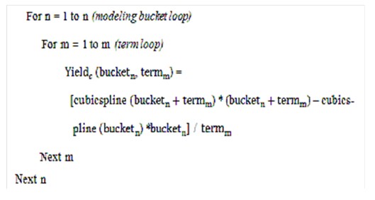
Description of the process to determine the implied forward rates follows
In the earlier formula, cubic spline refers to the cubic spline function. This function, currently used in the Rate Generator for Monte Carlo, takes a term as an argument and returns the smoothed yield for that term.
5. Translate continuous yields to discrete yields.
The output of the formula mentioned earlier produces a continuous yield, referred to as Yieldc. The required format for yield is a discrete yield. To translate from the continuous yield to the discrete yield (Yieldd), the following formula must be applied:
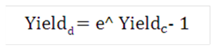
Description of the formula of discrete yield calculation follows
For Change From Base interest rate forecasting, the base scenario is calculated first and then the incremental change is applied to all rates.
For the Yield Curve Twist forecasting method, the user must select 3 term points to represent the following:
Short Point: This can be the first tenor from the yield curve, but can also be an intermediate point.
Anchor Point: The anchor point is typically the point on the yield curve where the pivot occurs. It typically does not change in a twisted scenario.
Long Point: The long point can be the last tenor in the yield curve or an intermediate point.
If intermediate points are selected for either the short point or the long point, all term points less than the short point and greater than the long point will reflect the same change amount input for the short and long points.
In addition to the six methods of IRC forecasting there are six shocks as part of the Basel Committee IRRBB Standardized Approach:
· Parallel Up and Down
· Short Rates Up and Down
· Flattener
· Steeper
A Long Rate shock is also applied as part of the Standardized Approach, but this is an interim, reference-only shock needed for the steeper and flattener scenarios. Also, scenario 1 of a Forecast Rates rule will always serve as the base rate scenario to which these shocks will be applied.
Standardized Approach (SA) shocks are an integral part of the larger Standardized Approach for IRRBB solution. Standardized Approach shocks have special application and therefore are scenario-level rules in Forecast Rates and apply to a limited number of currencies as prescribed by the Basel IRRBB publication. Appendix C “The Standardized Approach in IRRBB” contains the general framework to the solutions provided by the ALM Application. Also see the Basel Committee on Banking Supervision’s publication “Interest rate risk in the banking book”, Annex 2 “The standardized interest rate shock scenarios” for further details and applicable usage guidance.
For applicable IRC currencies, the rate changes represent instantaneous shocks that are held constant over the life of the forecast and are calculated. Standardized Approach formula constants are stored in the table FSI_IRC_STDAPRCH_SHOCKS.

Description of the formula to calculate SA Parallel Up and Down follows
Where Delta R for the parallel shift, for currency c on tenor (tk) is equal to the parallel up & down R-bar IRRBB-specified shock amount by currency.

Description of formula to calculate SA Short Up and Down follows

Description of formula to calculate SA Short Up and Down follows
Where Delta R short shock for currency c on tenor (tk) is equal to the up or down R-bar rate in basis points by currency times the Sshort scaling factor on tenor (tk), which is equal to the natural exponent of the quantity of the negative yield curve tenor length in years (tk), divided by x = 4. The constant x, as with other SA shock formula constants, are stored in FSI_IRC_STDAPRCH_SHOCKS.
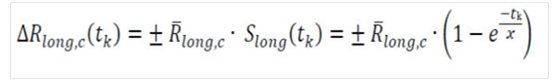
Where Delta R long shock for currency c on tenor (tk) is equal to the up or down R-bar long rate in basis points by currency times the Slong scaling factor on tenor (tk), which is equal to the one minus the natural exponent of the quantity of the negative yield curve tenor length in years (tk), divided by x = 4. Note that this is the additive inverse of the short rate scaling factor.
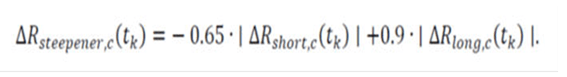
Description of formula to calculate SA Steepener Shock follows
Where Delta R steepener shock for currency c on tenor (tk) is equal to -.65 times the absolute value of the Delta R Short plus .9 times the absolute value of the Delta R Long rate. The Delta R Short and Delta R Long are the same values for the same currencies and tenors, as calculated in their respective shocks as described above. Formula constants above are stored in the table: FSI_IRC_STDAPRCH_SHOCKS.
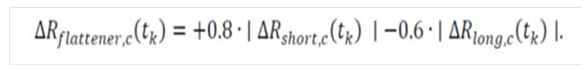
Description of formula to calculate SA Flattener Shock follows
Where Delta R flattener shock for currency c on tenor (tk) is equal to .8 times the absolute value of the Delta R Short plus -.6 times the absolute value of the Delta R Long rate. The Delta R Short and Delta R Long are the same values for the same currencies and tenors, as calculated in their respective shocks as described above. Standardized Approach shocks scaling factors for CPR & ER are stored in the table FSI_IRC_STDAPRCH_CPRER.