This chapter describes the option cost calculations implemented in Oracle Funds Transfer Pricing, including a theoretical overview, the mathematical details of the calculations, and examples.
Topics:
· Overview of Transfer Pricing Option Costs
· Theory
The purpose of option cost calculations is to quantify the cost of optionality, in terms of a spread over the transfer rate, for a single instrument. The cash flows of an instrument with an optionality feature change under different interest rate environments and thus should be priced accordingly.
For example, many mortgages may be prepaid by the borrower at any time without penalty. In effect, the lender has granted the borrower an option to buy back the mortgage at par, even if interest rates have fallen in value. Thus, this option has value.
In another case, an adjustable-rate loan may be issued with rate caps (floors) that limit it's maximum (minimum) periodic cash flows. These caps and floors constitute options. For the lender, the option cost of a cap is positive and negative for a floor.
Such flexibility given to the borrower raises the bank's cost of funding the loan and affects the underlying profit. The calculated cost of these options may be used in conjunction with the transfer rate to analyze profitability.
Oracle Funds Transfer Pricing uses the Monte Carlo methodology to calculate option costs. This methodology is described in Monte Carlo Analytics in the context of Oracle Asset Liability Management (ALM). Although Monte Carlo simulation in Oracle ALM generates different types of results than in Transfer Pricing, the underlying calculations are very similar.
In Oracle Funds Transfer Pricing, the option cost is calculated indirectly. Oracle Funds Transfer Pricing calculates and outputs two spreads:
· static spread
· option-adjusted spread (OAS)
The option cost is defined by:
· option cost = static spread – OAS
In the theory section, we show that the static spread is equal to margin (credit spread) and the OAS to the risk-adjusted margin of an instrument. Therefore, the option cost quantifies the loss or gain due to risk.
For clarity, this chapter assumes the following:
The instrument pays K cash flows occurring each at the end of the month.
Each month has the same duration, in the number of years, such as 1/12.
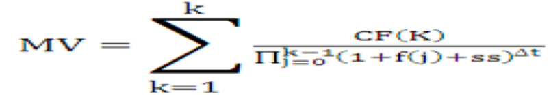
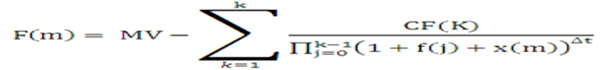
Neither the static spread nor the OAS can be defined directly as they are solutions of two different equations. We give hereafter a simplified version of the equations that the system solves, using the assumptions described earlier. The static spread is the value ss that solves the following equation:
Equation 1
Description of the Transfer Pricing Option Cost Equation 1 follows
Where:
:MV |
market, or book, or par value of the instrument (as selected in the Transfer Pricing rule) |
CF(k) |
cash flow occurring at the end of month k along with the forward rate scenario |
:f(j) |
forward rate for month j |
∆t |
length (in years) of the compounding period; hard-coded to a month, such as 1/12 |
In the Monte Carlo methodology, the option adjusted-spread is the value OAS that solves the following equation:
Equation 2

Description of the Transfer Pricing Option Cost Equation 2 follows
Where:
: N |
total number of Monte Carlo scenarios |
CF(K,ω) |
cash flow occurring at the end of month k along scenario ω |
D(k, ω,OAS) |
fstochastic discount factor at the end of month k along scenario ω for a particular OAS |
Note that:
· Cash flows are calculated up till maturity even if the instrument is adjustable.
NOTE |
Otherwise, the calculations would not catch the cost of caps or floors. |
· In the real calculations, the formula for the stochastic discount factor is simplified.
In this example, the Transfer Pricing curve is the Treasury curve. It is flat at 5%, which means that the forward rate is equal to 1%. We use only two Monte Carlo scenarios:
· up scenario: 1-year rate one year from now equal to 6%.
· down scenario: 1-year rate one year from now equal to 5%.
Observe that the average of these 2 stochastic rates is equal to 5%.
The instrument record is 2 years adjustable, paying yearly, with simple amortization. Its rate is Treasury plus 2%, with a cap at 7.5%. The par value and market value are equal to $1.
For simplicity in this example we assume that the compounding period used for discounting is equal to a year, for example:
Equation 3

Description of the Transfer Pricing Option Cost Equation 3 follows
The static spread is the solution to the following equation:
Equation 4
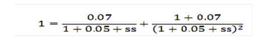
Description of the Transfer Pricing Option Cost Equation 4 follows
It is intuitively obvious that the static spread should be equal to the margin, for example:
NOTE |
We prove this claim in the Theory section of this chapter. |
static spread = coupon rate - forward rate= 7%-5%=2%.
Plugging this value in the right side of the earlier equation yields:
Equation 5
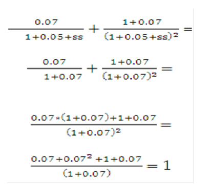
Description of the Transfer Pricing Option Cost Equation 5 follows
This is equal to par.
The OAS is the solution to the following equation:
Equation 6

Description of the Transfer Pricing Option Cost Equation 6 follows
Description of the Transfer Pricing Option Cost Equation 6 follows
By trial and error, we find a value of 1.88%. To summarize:
option cost = static spread - OAS=2%-1.88%=12 bp
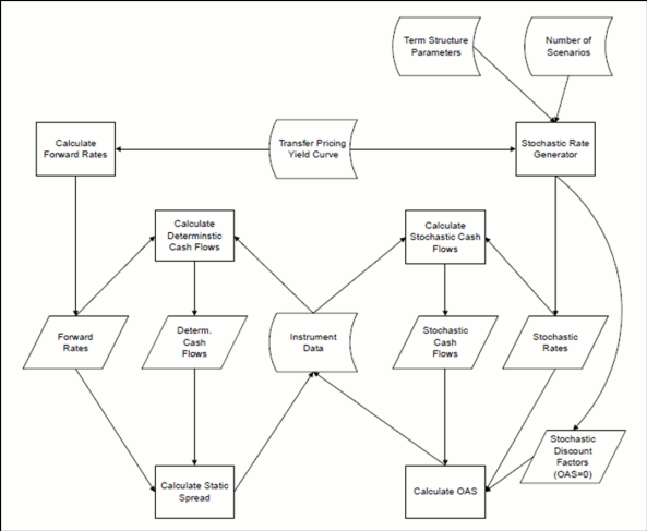
In this section we describe only the following steps:
· Calculate forward rates
· Calculate static spread
· Calculate OAS
The other steps are described later.
The cubic spline interpolation routine first calculates smoothed continuously compounded zero-coupon yields Y(j) with maturity equal to the end of month j. The formula for the one-month annually compounded forward rate spanning month j+1 is:
Equation 7
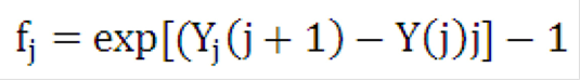
Description of the Transfer Pricing Option Cost Equation 7 follows
The static spread is calculated using the Newton-Raphson algorithm. If the Newton-Raphson algorithm does not converge, we revert to a brute search algorithm, which is much slower.
NOTE |
This can happen if cash flows alternately in sign. |
The user can control the convergence speed of the algorithm by adjusting the value of the variable Option Cost Speed Factor. This variable is defined in the Oracle FTP Application Preferences screen.
The default value is equal to one. A lower speed factor results in better accuracy of the results :
NOTE |
In all our experiments, a speed factor equal to one resulted in a maximum error (on the static spread and OAS) lower than half a basis point. |
For convenience, we recap hereafter Newton's algorithm. Let x be the static spread. At each iteration m we define the function F(m) by the following equation:
Equation 8
Description of the Transfer Pricing Option Cost Equation 8 follows
The algorithm is:
Equation 9
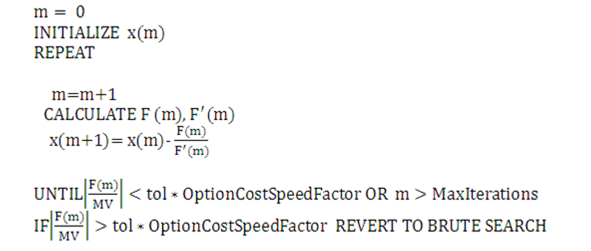
Description of the Transfer Pricing Option Cost Equation 9 follows
For performance reasons, the code uses a more complicated algorithm albeit similar in spirit than the one described earlier. This is the reason why we did not give specific values for tol (tolerance) and Max Iterations or details on the brute search.
For fixed-rate instruments, such as instruments for which the deterministic cash flows are the same as the stochastic cash flows, the OAS is by definition equal to the static spread.
NOTE |
This statement is true in the case of continuous compounding. For discrete compounding, this approximation has a negligible impact on the accuracy of the results. |
The OAS is also calculated with an optimized version of the Newton-Raphson algorithm. To get a gist of the Newton-Raphson method, see the previous section, with the following substitutions:
Equation 10
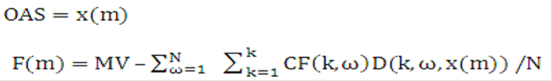
Description of the Transfer Pricing Option Cost Equation 10 follows
In this section, we show that the static spread is equal to margin and the OAS to the risk-adjusted margin of an instrument when the user selects the market value of the instrument to equate the discounted stream of cash flows. We assume in this section that the reader has a good knowledge of the no-arbitrage theory.
We first need some assumptions and definitions
· To acquire the instrument, the bank pays an initial amount V(0), the current market value.
· The risk-free rate is denoted by r(t).
· The instrument receives a cash flow rate equal to C(t), with 0≤ t ≤ T. (= maturity)
· The bank reinvests the cash flows in a money market account that, with the instrument, composes the portfolio.
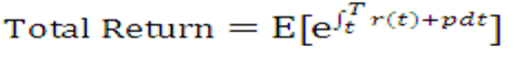
· The total return on a portfolio is equal to the expected future value divided by the initial value of the investment.
· The margin p on a portfolio is the difference between the rate of return (used to calculate the total return) and the risk-free rate r.
· The risk-adjusted expected future value of a portfolio is equal to its expected future value after hedging all diversifiable risks.
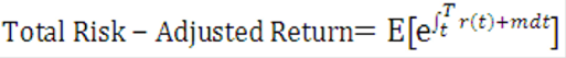
· The total risk-adjusted return of a portfolio is equal to the risk-adjusted expected future value divided by the initial value of the investment.
· The risk-adjusted margin m of a portfolio is the difference between the risk-adjusted rate of return (used to calculate the total risk-adjusted return) and the risk-free rate r.
More precisely,
Equation 11
Description of the Transfer Pricing Option Cost Equation 11 follows
Equation 12
Description of the Transfer Pricing Option Cost Equation 12 follows
In a no-arbitrage economy with complete markets, the market value at time t of an instrument with cash flow rate C(t) is given by:
Equation 13

Description of the Transfer Pricing Option Cost Equation 13 follows
and expectation is taken concerning the risk-neutral measure. The expected change in value is given by:
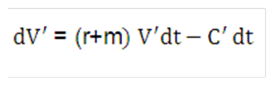
Equation 14
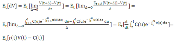
Description of the Transfer Pricing Option Cost Equation 14 follows
The variation in value is therefore equal to the expected value of the change dV plus the change in the value of a martingale M in the risk-neutral measure:
Equation 15

Description of the Transfer Pricing Option Cost Equation 15 follows
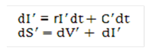
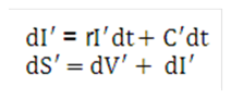
Let I be the market value of the money market account in which cash flows are reinvested.
Equation 16
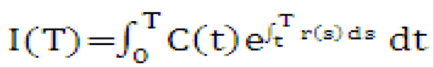
Description of the Transfer Pricing Option Cost Equation 16 follows
Note that unlike V this is a process of finite variation. By Ito's lemma,
Equation 17

Description of the Transfer Pricing Option Cost Equation 17 follows
Let S be the market value of a portfolio composed of the instrument plus the money market account. We have:
Equation 18
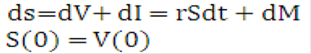
Description of the Transfer Pricing Option Cost Equation 18 follows
In other terms, the portfolio (and not the instrument) earns the risk-free rate of return. An alternate representation of this process is:
Equation 19
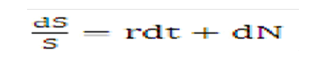
Description of the Transfer Pricing Option Cost Equation 19 follows
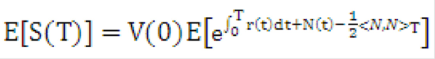
where N is another martingale in the risk-neutral measure. The expected value of the portfolio is then:
Equation 20
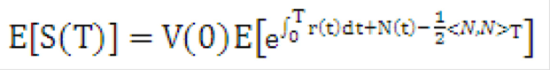
Description of the Transfer Pricing Option Cost Equation 20 follows
Where
<N,N>
is the quadratic variation of N. This is equivalent to:
Equation 21
Description of the Transfer Pricing Option Cost Equation 21 follows
Let us define the martingale:
Equation 22
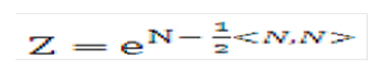
Description of the Transfer Pricing Option Cost Equation 22 follows
This represents the relative risk of the portfolio for the standard money market account, that is, the account where only an initial investment of V(0) is made. Then,
Equation 23
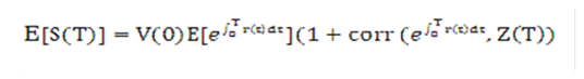
Description of the Transfer Pricing Option Cost Equation 23 follows
In other terms, the expected future value of the portfolio is equal to the expected future value of the money market account adjusted by the correlation between the standard money market account and the relative risk. Assuming complete and efficient markets, banks can fully hedge their balance sheet against this relative risk, which should be neglected to calculate the contribution of a particular portfolio to the profitability of the balance sheet. Therefore,
Equation 24
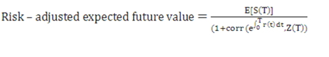
Description of the Transfer Pricing Option Cost Equation 24 follows
Equation 25
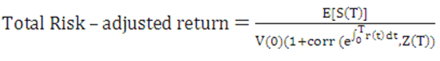
Description of the Transfer Pricing Option Cost Equation 25 follows
In this example, the risk-adjusted rate of return of the bank on its portfolio is equal to the risk-free rate of return.
Let us suppose now that another instrument offers cash flows
C'>C
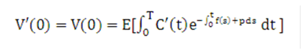
Assuming complete and efficient markets its market value will then be:
Equation 26

Description of the Transfer Pricing Option Cost Equation 26 follows
The value of the corresponding portfolio is denoted by
S'>S
By analogy with the previous development, we have:
Equation 27
Description of the Transfer Pricing Option Cost Equation 27 follows
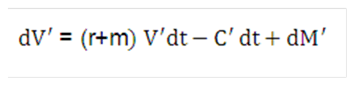
Again, the risk-adjusted rate of return of the bank on its portfolio is equal to the risk-free rate of return. Suppose now that markets are not complete and inefficient. The bank pays the value V(0) and receives cash flows equal to C'. We have:
Equation 28
Description of the Transfer Pricing Option Cost Equation 28 follows
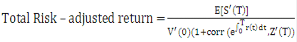
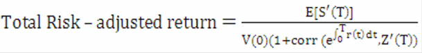
By definition of the total risk-adjusted return, we have:
Equation 29
Description of the Transfer Pricing Option Cost Equation 29 follows
Therefore, by analogy with the previous development,
Equation 30
Description of the Transfer Pricing Option Cost Equation 30 follows
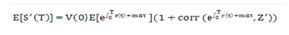
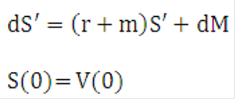
This can be decomposed into
Equation 31
Description of the Transfer Pricing Option Cost Equation 31 follows
Equation 32
Description of the Transfer Pricing Option Cost Equation 32 follows
Equation 33

Description of the Transfer Pricing Option Cost Equation 33 follows
The solution of Equation 31 and Equation 33 is:
Equation 34
Description of solution for the Transfer Pricing Option Cost Equation 31 and 33 follows
By the law of large numbers, Equation 31 and Equation33 result in:
Equation 35
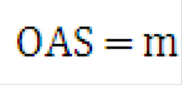
Description of the Transfer Pricing Option Cost Equation 35 follows
For example, the OAS is equal to the risk-adjusted margin.
Static spread calculations are deterministic, therefore they are a special case of the equations in the previous section where, roughly speaking, all processes are equal to their expected value, and the margin p is substituted to the risk-adjusted margin m. The equivalent of �Equation 8–29 is then
Equation 36

Description of the Transfer Pricing Option Cost Equation 36 follows
Where f is the instantaneous forward rate. The equivalent of Equation 8–31 and Equation 8–33 is then
Equation 37
Description of the Transfer Pricing Option Cost Equation 37 follows
Equation 38
Description of the Transfer Pricing Option Cost Equation 38 follows
Equation 39

Description of the Transfer Pricing Option Cost Equation 39 follows
The solution of Equation 37 and Equation 39 is:
Equation 40

Description of the Transfer Pricing Option Cost Equation 40 follows
Comparing Equation40 and Equation 8:
Equation 41

Description of the Transfer Pricing Option Cost Equation 41 follows
For example, the static spread is equal to the margin.
In some very rare cases, there is more than one value that solves the static spread equation. This section describes one of these cases.
The market value of the instrument is $0.445495. It has 2 cash flows. The following table shows the value of the cash flows and corresponding discount factors (assuming a static spread of zero).
|
First event |
Second event |
Time |
1 |
2 |
Cash flow value |
1 |
-0.505025 |
Discount factor(static spread=0) |
0.9 |
0.8 |
The continuously compounded static spread solves the following equation:
Equation 42
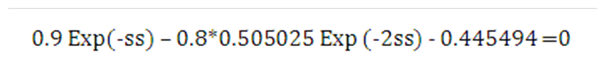
Description of the Transfer Pricing Option Cost Equation 42 follows
There are two possible solutions for the static spread:
static spread =0.19%
static spread =1.81$
In case you desire a better numerical precision than the default precision, you can take two actions:
· Decrease the speed factor (see the section Calculate Static Spread).
· Increase the number of Monte Carlo scenarios.
Both actions increase calculation time.