Pg2vec
Overview of the algorithm
Pg2vec learns representations of graphlets (partitions inside a graph) by employing edges as the principal learning units and thereby packing more information
in each learning unit (as compared to previous approaches employing vertices as learning units) for the representation
learning task. It consists of three main steps:
We generate random walks for each vertex (with pre-defined length per walk and pre-defined number of walks per vertex).
Each edge in this random walk is mapped as a
property edge-wordin the created document (with the document label as the graph-id) where the property edge-word is defined as the concatenation of the properties of the source and destination vertices.We feed the generated documents (with their attached document labels) to a doc2vec algorithm which generates the vector representation for each document (which is a graph in this case).
Pg2vec creates graphlet embeddings for a specific set of graphlets and cannot be updated to incorporate modifications on these graphlets.
Instead, a new Pg2vec model should be trained on these modified graphlets.
Lastly, it is important to note that the memory consumption of Pg2vec model is O(2(n+m)*d) where n is
the number of vertices in the graph, m is the number of graphlets in the graph, and d is the embedding length.
Functionalities
We provide here the main functionalities for our implementation of Pg2vec in PGX
using NCI109 dataset as an example (with 4127 graphs in it).
Loading a graph
First, we create a session and an analyst:
1session = pypgx.get_session(session_name="my-session")
2analyst = session.create_analyst()
Our h algorithm can be applied to directed or undirected graphs
(even though we only consider undirected random walks). To begin with, we can load a graph as follows:
1graph = session.read_graph_with_properties(self.small_graph)
Building a Pg2vec Model (minimal)
We can build a Pg2vec model using the minimal configuration and default hyper-parameters as follows:
1model = analyst.pg2vec_builder(
2    graphlet_id_property_name="graph_id",
3    vertex_property_names=["category"],
4    window_size=4,
5    walks_per_vertex=5,
6    walk_length=8
7)
We specify the property name to determine each graphlet using the
Pg2vecModelBuilder.setGraphLetIdPropertyName() operation and also employ the vertex properties in Pg2vec which are specified using the Pg2vecModelBuilder.setVertexPropertyNames() operation.
We can also use the weakly connected component (WCC) functionality in PGX to determine the graphlets in a given graph.
Building a Pg2vec Model (customized)
We can build a Pg2vec model using customized hyper-parameters as follows:
 1model = analyst.pg2vec_builder(
 2    graphlet_id_property_name="graph_id",
 3    vertex_property_names=["category"],
 4    min_word_frequency=1,
 5    batch_size=128,
 6    num_epochs=5,
 7    layer_size=200,
 8    learning_rate=0.04,
 9    min_learning_rate=0.0001,
10    window_size=4,
11    walks_per_vertex=5,
12    walk_length=8,
13    use_graphlet_size=True,
14    graphlet_size_property_name="graphletSize-Pg2vec",
15)
We provide complete explanation for each builder operation (along with the default values) in our Pg2vecModelBuilder docs.
Training the Pg2vec model
We can train a Pg2vec model with the specified (default or customized) settings as follows:
1model.fit(graph)
Getting the loss value
We can fetch the loss value on a specified fraction of training data as follows:
1loss = model.loss
Computing the similar graphlets
We can fetch the k most similar graphlets for a given graphlet with the following code:
1similars = model.compute_similars(1, 10)
The output results will be in the following format, for e.g., searching for similar vertices for graphlet with ID = 52 using
the trained model:
dstGraphlet |
similarity |
|---|---|
52 |
1.0 |
10 |
0.8748674392700195 |
23 |
0.8551455140113831 |
26 |
0.8493421673774719 |
47 |
0.8411962985992432 |
25 |
0.8281504511833191 |
43 |
0.8202780485153198 |
24 |
0.8179885745048523 |
8 |
0.796689510345459 |
9 |
0.7947834134101868 |
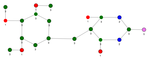
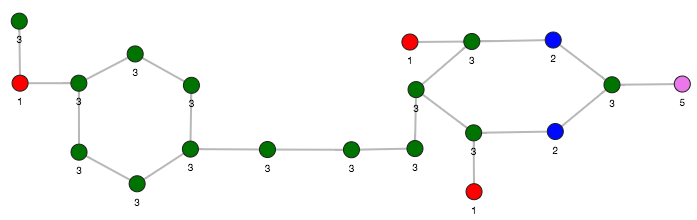
The visualization of two similar graphlets (top: ID = 52 and bottom: ID = 10).
Computing the similars (for a graphlet batch)
We can fetch the k most similar graphlets for a batch of input graphlets with the following code:
1batched_similars = model.compute_similars([1, 2], 10)
The output results will be in the following format, for e.g., searching for similar vertices for graphlets
with ID = 52 and ID = 41 using the trained model.
srcGraphlet |
dstGraphlet |
similarity |
|---|---|---|
52 |
52 |
1.0 |
52 |
10 |
0.8748674392700195 |
52 |
23 |
0.8551455140113831 |
52 |
26 |
0.8493421673774719 |
52 |
47 |
0.8411962985992432 |
52 |
25 |
0.8281504511833191 |
52 |
43 |
0.8202780485153198 |
52 |
24 |
0.8179885745048523 |
52 |
8 |
0.796689510345459 |
52 |
9 |
0.7947834134101868 |
41 |
41 |
1.0 |
41 |
197 |
0.9653506875038147 |
41 |
84 |
0.9552277326583862 |
41 |
157 |
0.9465565085411072 |
41 |
65 |
0.9287481307983398 |
41 |
248 |
0.9177336096763611 |
41 |
315 |
0.9043129086494446 |
41 |
92 |
0.8998928070068359 |
41 |
297 |
0.8897411227226257 |
41 |
50 |
0.8810243010520935 |
Inferring a graphlet vector
We can infer the vector representation for a given new graphlet with the following code:
1from pypgx.api.filters import VertexFilter
2graphlet = graph.filter(VertexFilter("vertex.graph_id = 1"))
3inferred_vector = model.infer_graphlet_vector(graphlet)
4inferred_vector.print()
The schema for the inferred_vector would be as follows:
graphlet |
embedding |
Inferring vectors (for a graphlet batch)
We can infer the vector representations for multiple graphlets (specified with different graph-ids in a graph) with the following code:
1graphlets = session.read_graph_with_properties(
2    self.small_graph
3)
4inferred_vector_batched = model.infer_graphlet_vector_batched(
5    graphlets
6)
7inferred_vector_batched.print()
The schema is same as for inferGraphletVector but with more rows corresponding to the input graphlets.
Getting all trained graphlet vectors
We can retrieve the trained graphlet vectors for the current Pg2vec model as follows:
1vertex_vectors = model.trained_graphlet_vectors.flatten_all()
2vertex_vectors.store(
3    path=tmp + "/graphlet_vectors.tsv",
4    overwrite=True,
5    file_format="csv"
6)
The schema is the same as for inferGraphletVector but with more rows corresponding to all the graphlets in the input graph.
Storing a trained model
Models can be stored either to the server file system, or to a database.
The following shows how to store a trained Pg2vec model to a specified file path:
1model.export().file(path=tmp + "/model.model", key="test", overwrite=True)
When storing models in database, they are stored as a row inside a model store table.
The following shows how to store a trained Pg2vec model in database in a specific model store table:
1model.export().db(
2    username="user",
3    password="password",
4    model_store="modelstoretablename",
5    model_name="model",
6    jdbc_url="jdbc_url"
7)
Loading a pre-trained model
Similarly to storing, models can be loaded from a file in the server file system, or from a database.
It is possible to load a pre-trained Pg2vec model from a specified file path as follows:
1analyst.get_pg2vec_model_loader().file(
2    path=tmp + "/model.model",
3    key="test"
4)
We can load a pre-trained Pg2vec model from a model store table in database as follows:
1analyst.get_pg2vec_model_loader().db(
2    username="user",
3    password="password",
4    model_store="modelstoretablename",
5    model_name="model",
6    jdbc_url="jdbc_url"
7)
Destroying a model
We can destroy a model with the following operation:
1model.destroy()