Example: Method 7: Second Degree Approximation

Linear Regression determines values for a and b in the forecast formula Y = a + b X with the objective of fitting a straight line to the sales history data. Second Degree Approximation is similar, but this method determines values for a, b, and c in the this forecast formula:

Y = a + b X + c X²

The objective of this method is to fit a curve to the sales history data. This method is useful when a product is in the transition between life cycle stages. For example, when a new product moves from introduction to growth stages, the sales trend might accelerate. Because of the second order term, the forecast can quickly approach infinity or drop to zero (depending on whether coefficient c is positive or negative). This method is useful only in the short term.

Forecast specifications: the formula find a, b, and c to fit a curve to exactly three points. You specify n, the number of time periods of data to accumulate into each of the three points. In this example, n = 3. Actual sales data for April through June is combined into the first point, Q1. July through September are added together to create Q2, and October through December sum to Q3. The curve is fitted to the three values Q1, Q2, and Q3.

Required sales history: 3 × n periods for calculating the forecast plus the number of time periods that are required for evaluating the forecast performance (periods of best fit).

This table is history used in the forecast calculation:

Past Year	Jan	Feb	Mar	Apr	May	Jun	Jul	Aug	Sep	Oct	Nov	Dec
1	None	None	None	125	122	137	140	129	131	114	119	137

Q0 = (Jan) + (Feb) + (Mar)

Q1 = (Apr) + (May) + (Jun) which equals 125 + 122 + 137 = 384

Q2 = (Jul) + (Aug) + (Sep) which equals 140 + 129 + 131 = 400

Q3 = (Oct) + (Nov) + (Dec) which equals 114 + 119 + 137 = 370

The next step involves calculating the three coefficients a, b, and c to be used in the forecasting formula Y = a + b X + c X².

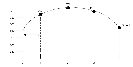
Q1, Q2, and Q3 are presented on the graphic, where time is plotted on the horizontal axis. Q1 represents total historical sales for April, May, and June and is plotted at X = 1; Q2 corresponds to July through September; Q3 corresponds to October through December; and Q4 represents January through March. This graphic illustrates the plotting of Q1, Q2, Q3, and Q4 for second degree approximation:

Three equations describe the three points on the graph:

(1) Q1 = a + bX + cX² where X = 1(Q1 = a + b + c)

(2) Q2 = a + bX + cX² where X = 2(Q2 = a + 2b + 4c)

(3) Q3 = a + bX + cX² where X = 3(Q3 = a + 3b + 9c)

Solve the three equations simultaneously to find b, a, and c:

1. Subtract equation 1 (1) from equation 2 (2) and solve for b:

   (2) – (1) = Q2 – Q1 = b + 3c

   b = (Q2 – Q1) – 3c

2. Substitute this equation for b into equation (3):

   (3) Q3 = a + 3[(Q2 – Q1) – 3c] + 9c a = Q3 – 3(Q2 – Q1)

3. Finally, substitute these equations for a and b into equation (1):

   (1)[Q3 – 3(Q2 – Q1)] + [(Q2 – Q1) – 3c] + c = Q1

   c = [(Q3 – Q2) + (Q1 – Q2)] / 2

The Second Degree Approximation method calculates a, b, and c as follows:

a = Q3 – 3(Q2 – Q1) = 370 – 3(400 – 384) = 370 – 3(16) = 322

b = (Q2 – Q1) –3c = (400 – 384) – (3 × –23) = 16 + 69 = 85

c = [(Q3 – Q2) + (Q1 – Q2)] / 2 = [(370 – 400) + (384 – 400)] / 2 = –23

This is a calculation of second degree approximation forecast:

Y = a + bX + cX² = 322 + 85X +(–23) (X²)

When X = 4, Q4 = 322 + 340 – 368 = 294. The forecast equals 294 / 3 = 98 per period.

When X = 5, Q5 = 322 + 425 – 575 = 172. The forecast equals 172 / 3 = 58.33 rounded to 57 per period.

When X = 6, Q6 = 322 + 510 – 828 = 4. The forecast equals 4 / 3 = 1.33 rounded to 1 per period.

This is the forecast for next year, Last Year to This Year:

Jan	Feb	Mar	Apr	May	Jun	Jul	Aug	Sep	Oct	Nov	Dec
98	98	98	57	57	57	1	1	1	NA	NA	NA