Formatting a pivot table and adding calculations
This tutorial shows you how to format a pivot table and add some calculations.
What you'll learn
In this tutorial, we'll show you how to:
- Format numbers in the pivot table
- Move some data in the pivot table to a row
- Add a calculation to the pivot table
- Change the display width of the pivot table
What you'll need
- Access to Insight
- Analyzer license
- Completed the tutorial Creating analysis with a pivot table
Step 1: Format numbers in the pivot table
First, we'll update a column to change the column name and the format of the column numbers.
To format numbers:
- Open the analysis you were working with in Creating analysis with a pivot table.
- Click
 Optionsfor Attributed Revenue and select Column Properties.
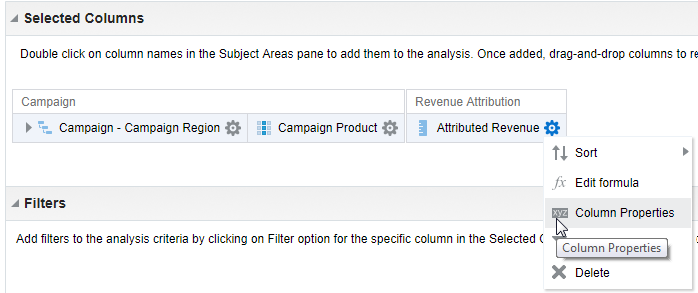
The Column Properties dialog box appears.
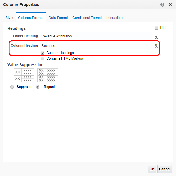
- Click the Column Format tab. Select the Custom Headings check box, and enter Revenue in the Column Heading field.
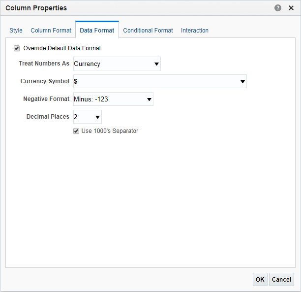
- Click the Data Format tab. Select the Override Default Data Format check box and select the values as indicated in the image below.
- Click OK and then click the Results tab.
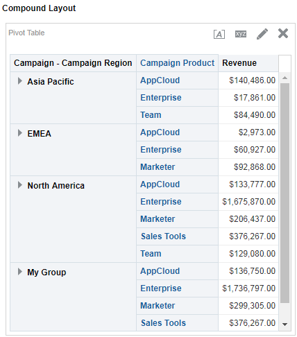
- Save your analysis.
Step 2: Changing the pivot table layout and adding calculations
In this step, you'll update the pivot table to move some of the data to columns instead of rows. You will also add a new calculation to the pivot table.
To change the pivot table layout and add a calculation:
- On the Results tab, click the
 Edit View to format the pivot table.
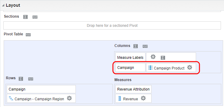
 - Use the Layout pane to format the pivot table. Drag Campaign Product below Measure Labels.
The Layout pane should look like this:
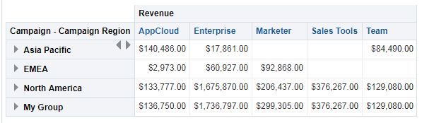
The pivot table now looks like this:
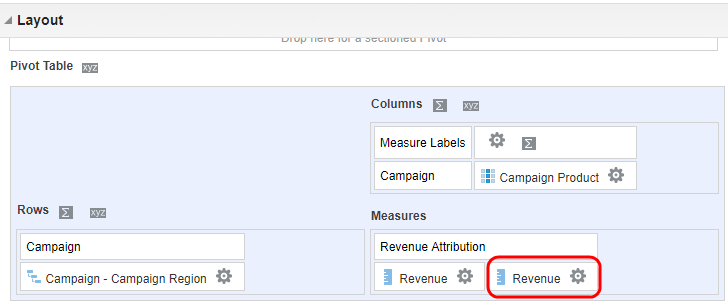
Next, add a calculation to the pivot table by duplicating the Revenue column.
- In the Layout pane, click More Options for the Revenue column and select Duplicate Layer.
The duplicated Revenue column appears.
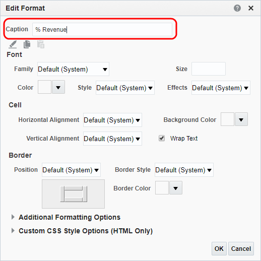
- For the duplicate Revenue column, click More Options > Format Heading.
The Edit Format dialog appears.
- Enter % Revenue in the Caption field, and click OK.
Next, we'll add a calculation to reflect a percentage of the parent.
- For the % Revenue column, click More Options > Show Data As > Percent of > Row Parent.
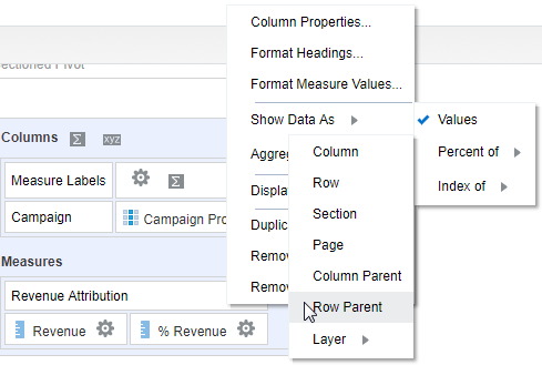
The calculation is added to the column.
Because we added these additional columns, the pivot table now has a horizontal scroll bar. Let's update the pivot table to increase the width.
- Click
 View Properties above the pivot table.
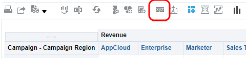
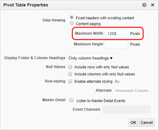
The Pivot Table Properties dialog appears.
- Enter 1200 in the Maximum Width field, and click OK.
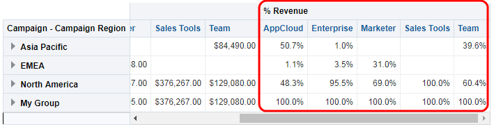
The pivot table now looks like this:
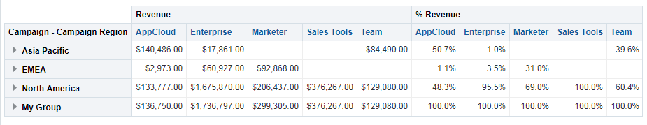
- Click Done and save the analysis.
Now that you're done
Oracle University offers the following instructor-led courses to help you achieve success:
- Oracle University - B2B: Insight for Analyzers
- Oracle University - B2B: Insight for Analyzers - Groups
- Oracle University - B2B: Insight for Analyzers - Dashboards
Also be sure to checkout the Oracle Business Intelligence Enterprise Edition Help Center where you can find more resources on using Oracle BI Enterprise Edition. Remember though, not all of the features included in a stand-alone version of Oracle BI EE are available in Insight.