Introduction
This tutorial supports customers and partners in configuring the Advanced Predictions with ML capability to generate more accurate predictions by considering key business drivers. This tutorial shows you how to configure Advanced Predictions and provides implementation recommendations based on business considerations and IPM's solution capabilities.This tutorial focuses on a specific business use case regarding Volume Forecasting and considering some key input drivers to train the ML model and generate more accurate predictions. The sections build on each other and should be completed sequentially.
Background
Advanced predictions or ML predictions refers to the process of using machine learning models to forecast data based on input features.
Key Benefits of Advanced Predictions:
- Enables more powerful predictions by correlating with other provided data points.
- Is embedded within Oracle EPM to empower finance & operational users with data science optimized for multidimensional planning & forecasting use cases.
- Leverages more sophisticated algorithms and improves accuracy.
- Configures more easily by using a step by step configuration wizard.
Advantages with Advanced Predictions:
- Grounded in your EPM data and context: Users don’t have to go to any external data science platform or ML tool. Advanced prediction capability is embedded within EPM data and context to empower finance and operational users.
- Powered by OCI AI infrastructure: build, train and deploy machine learning models within EPM systems.
- Privacy and security at every layer: Advanced prediction honors the EPM security layer which means access to prediction data generated by ML models is controlled by the same robust security framework that governs other areas of the EPM system.
- Embedded at no extra cost: Available with an Oracle EPM Enterprise license at no additional cost.
- Extensible framework: Supports processing and pre-processing of data, with an extensible framework using pipeline with external data, and supports prediction with multiple platforms using APIs, BYOML.
Key Considerations for Advanced Predictions:
- Available with Enterprise EPM license only
- Accessed only through the Redwood theme
- Is an opt-in only feature - opt-in available in Application Settings
- Embedded in EPM with OCI Data Science so there is no additional cost to deploy OCI Data Science
- Available in different Planning applications including Modules, Custom, FreeForm, Sales Planning, Strategic Workforce Planning, Predictive Cash Forecasting
- Works with both BSO and ASO cubes
Volume Forecasting Use Case
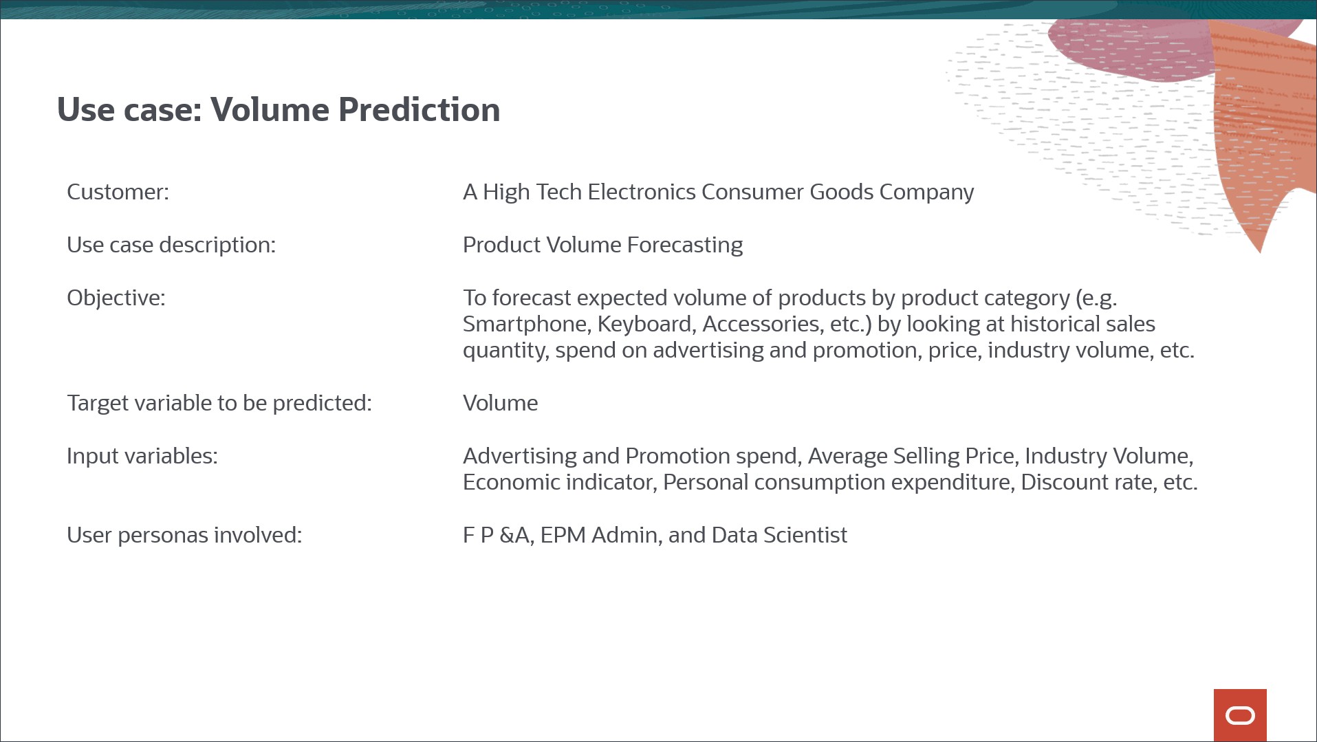
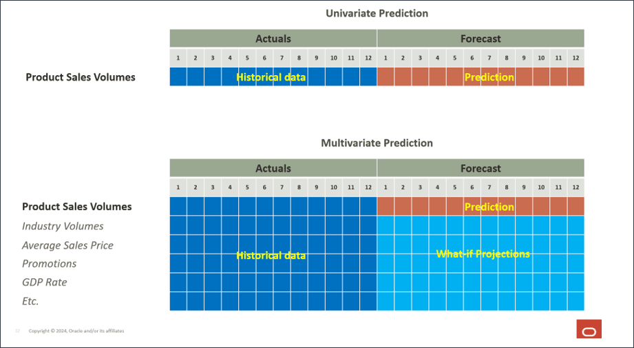
Consider the use case where you want to predict sales volume by product based on historical sales volumes from January FY22 to June FY24. In addition to historical sales volume, you also use input drivers such as industry volumes, average sales price, advertising and marketing promotions, and discount rate - all internal factors that can impact future volume prediction. You also use a couple of external drivers such as economic indicator such as GDP growth rate, and personal consumption expenditure that can have an impact on future volume prediction.
Historical input drivers are mostly imported from data sources, and future input driver values can be either planned using traditional methods like driver or trend-based, or you can use univariate prediction (imputation feature) available as part of the advanced prediction job itself.
Prerequisites
Cloud EPM Hands-on Tutorials may require you to import a snapshot into your Cloud EPM Enterprise Service instance. Before you can import a tutorial snapshot, you must request another Cloud EPM Enterprise Service instance or remove your current application and business process. The tutorial snapshot will not import over your existing application or business process, nor will it automatically replace or restore the application or business process you are currently working with.
Before starting this tutorial, you must:
- Have Service Administrator access to a Cloud EPM Enterprise Service instance. The instance should not have a business process created.
- Upload and import this snapshot into your Planning business process.
- Download this Date Mapping to your local machine.
Tip:
To save the file locally, you can right-click, and select Save Link As. Ensure you save the file as a .csv file. - Download this Sales Volume Forecast Report to your local machine.
Tip:
To save the file locally, you can right-click, and select Save Link As.
Note:
If you run into migration errors importing the snapshot, re-run the migration excluding the HSS-Shared Services component, as well as the Security and User Preferences artifacts in the Core component. For more information on uploading and importing snapshots, refer to the Administering Migration for Oracle Enterprise Performance Management Cloud documentation.Opting in for Advanced Predictions
If you want to start using Advanced predictions and AI capabilities, you need to first go to the Application Settings page and enable it.
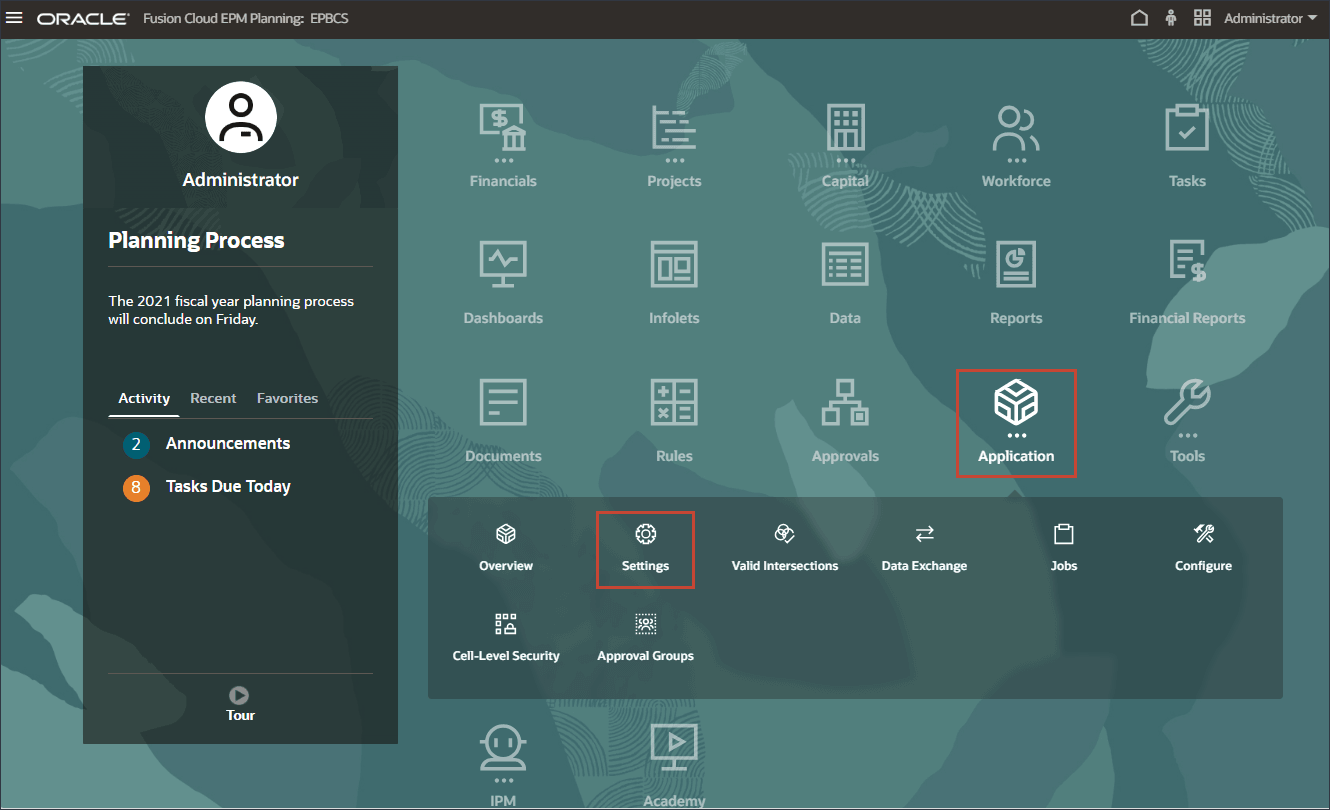
- On the home page, click Application, and then click Settings.
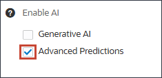
- In Settings, scroll down and in the lower right section, in Enable AI, select Advanced Predictions to enable AI data analysis for advanced, multivariate predictions.
- In the Information message, click OK.

- Scroll up and click Save.
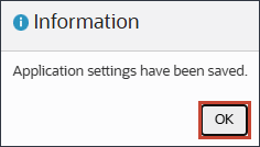
- In the Information message, click OK.
- Click
 (Home) to return to the Home page.
Preparing the Application
Before you perform the steps in this tutorial, you need to prepare the application. The provided application does not include groups, roles or security so you need to create the EPM group and then assign it to the EPM Cloud navigation flow. You use the EPM Cloud navigation flow to review the predictions generated using Advanced Predictions.
Creating the EPM Group
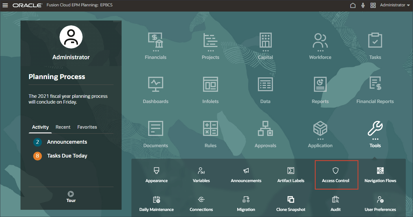
- On the home page, click Tools, and then click Access Control.
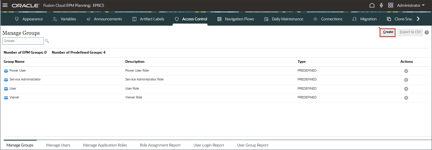
- In Manage Groups, click Create.
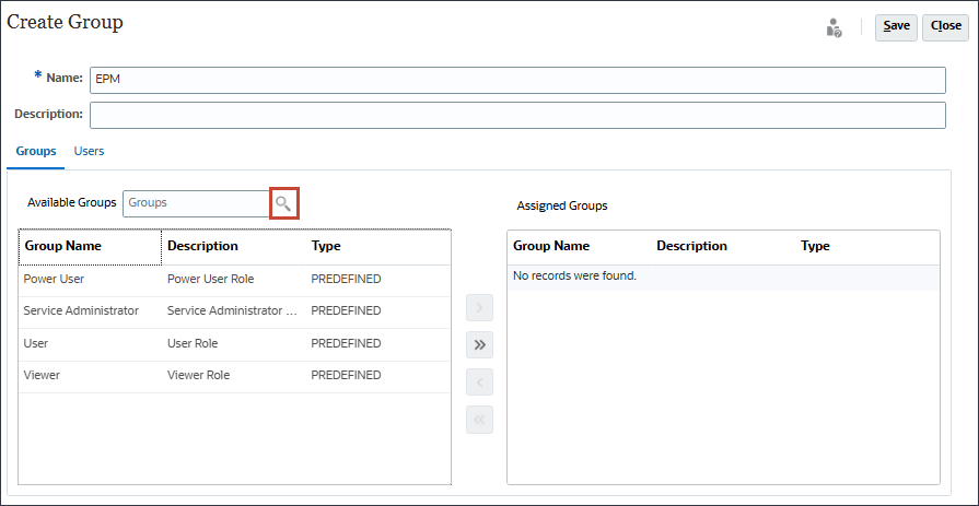
- In Create Group, for Name, enter EPM.
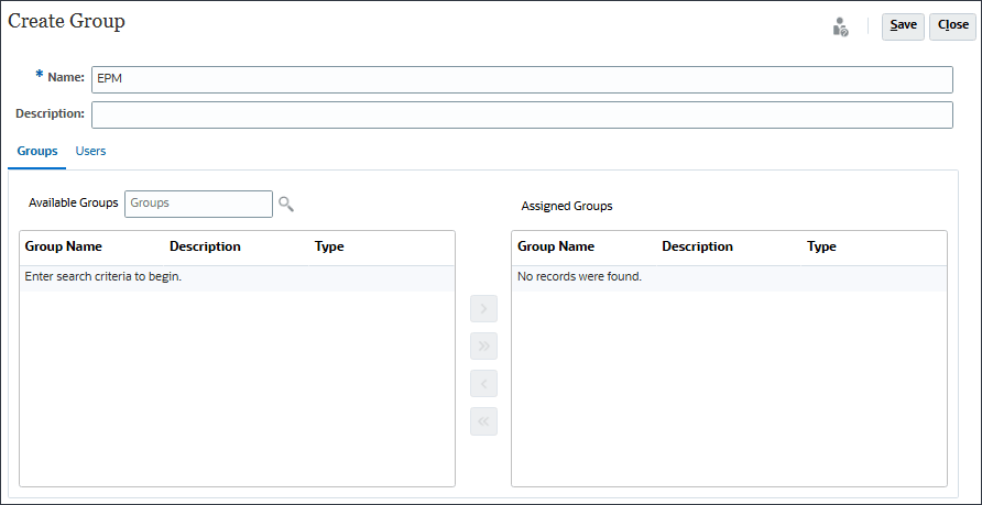
- With Groups selected, next to Available Groups, click
 (Search).
Available groups are listed.
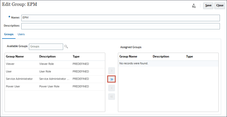
- To move all the predefined roles, click
 (Move All).
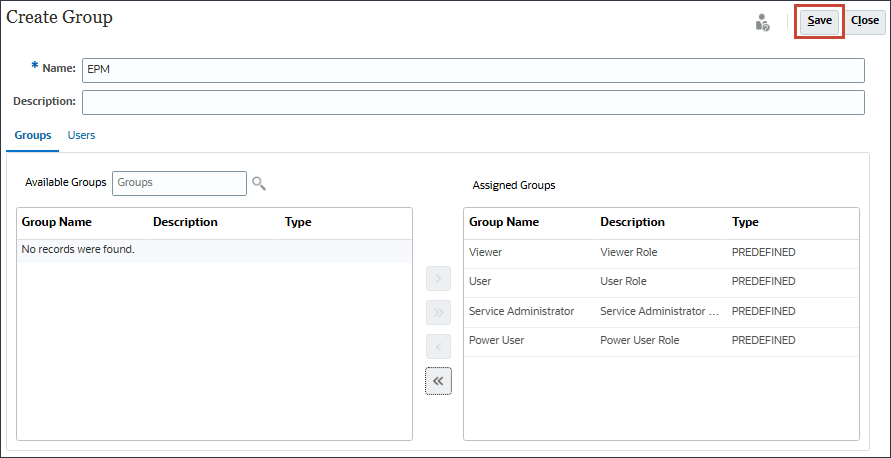
- Click Save.
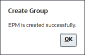
- At the information message, click OK.
- Verify that EPM is listed in Manage Groups.
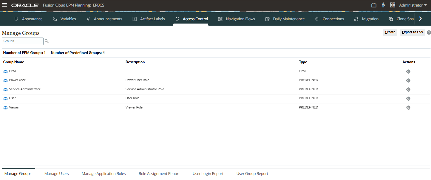
- Click
 (Home) to return to the Home page.
- On the home page, click Tools, and then click Navigation Flows.
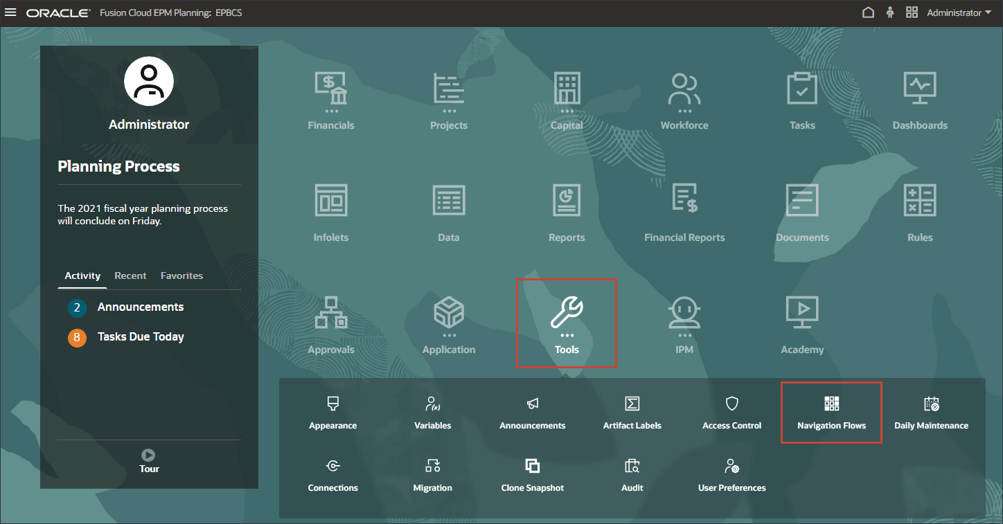
- In Navigation Flow, verify that EPM Cloud is set to Inactive, then click EPM Cloud.
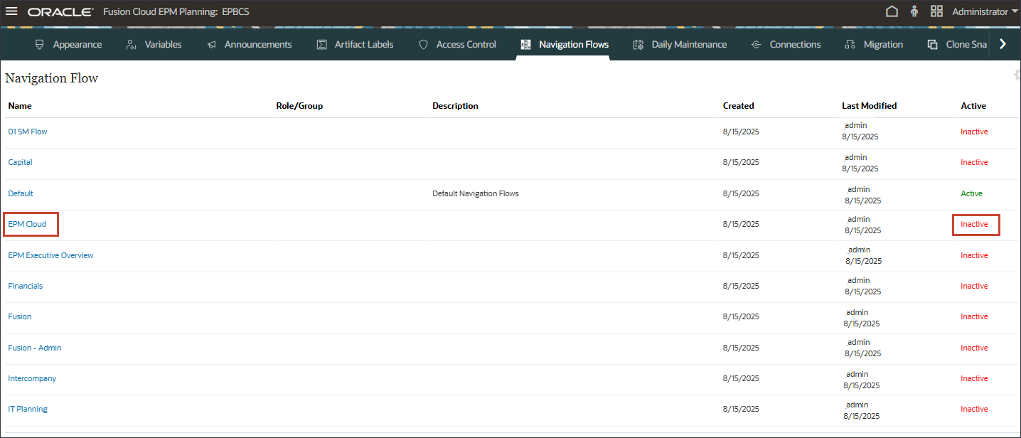
- In EPM Cloud, for Assign to, enter EPM, and click Save and Close.

- For EPM Cloud, click Inactive to activate the EPM Cloud navigation flow.

- Click
 (Home) to return to the Home page.
Assigning the EPM Group to the EPM Cloud Navigation Flow.
Preparing for Advanced Predictions
In this section, you complete end user steps before configuring advanced predictions. You ensure user variables are set and you select the EPM Cloud navigation flow. You also review the volume analysis dashboard. You review and edit input drivers. You review missing input driver values for future periods and you review the predictions form.
Setting User Variables
You set user variables so that you can view data in forms and dashboards.
- On the home page, click Tools, and then click User Preferences.
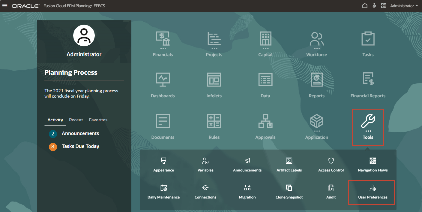
- Click User Variables.
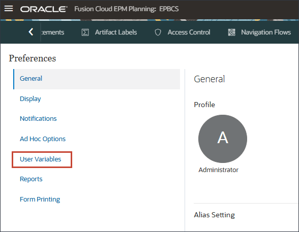
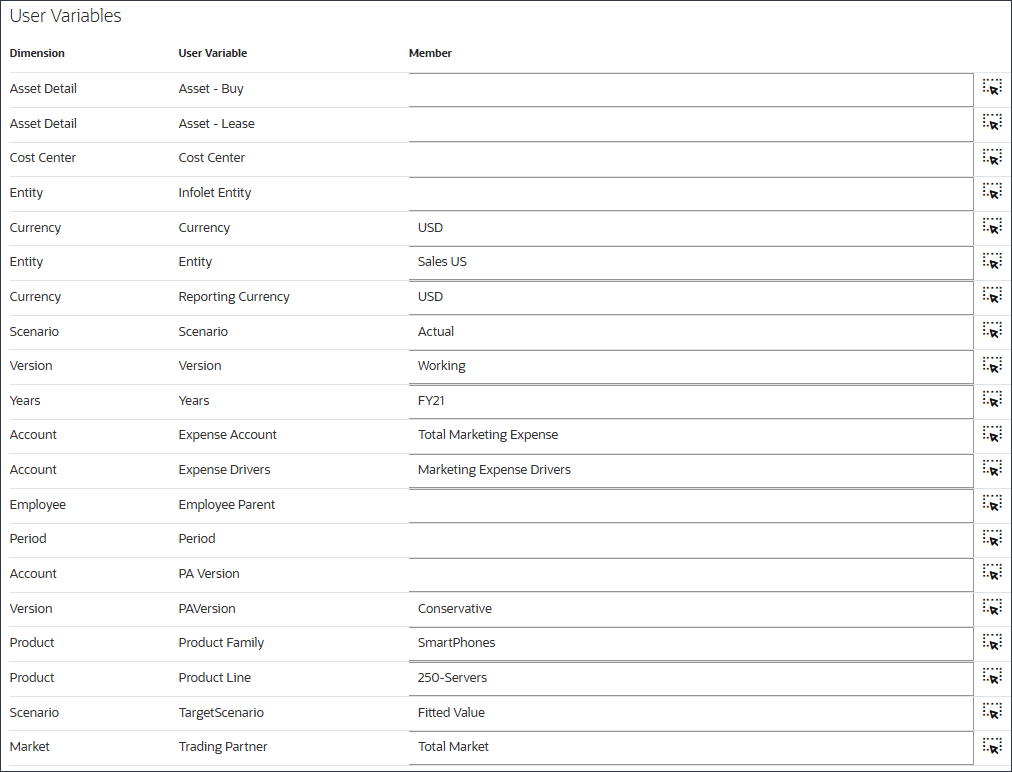
- For user variables, enter or select the following, and click Save.
Dimension User Variable Member Currency Currency USD Entity Entity Sales US Currency Reporting Currency USD Scenario Scenario Actual Version Version Working Years Years FY21 Account Expense Account Total Marketing Expense Account Expense Drivers Marketing Expense Drivers Version PA Version Conservative Product Product Family SmartPhones Product Product Line 250-Servers Scenario TargetScenario Fitted Value Market Trading Partner Total Market The user variables are selected.
- At the Information message, click OK.
- Click
 (Home) to return to the Home page.
Selecting Navigation Flow
You select the EPM Cloud navigation flow which includes a card for Advanced Predictions so you can review the volume forecast.
- On the home page, click
 (Default), and select EPM Cloud.
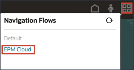
The EPM Cloud navigation flow is displayed.
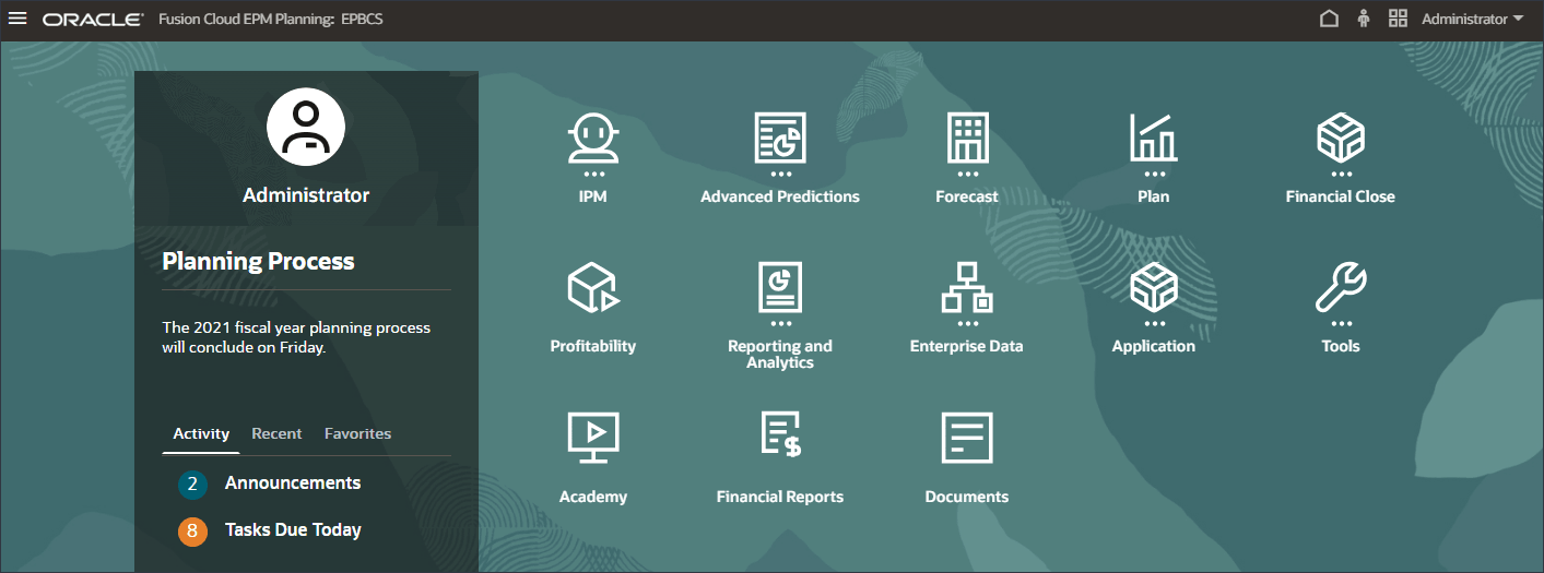
- In the EPM Cloud navigation flow, notice the Advanced Predictions card.
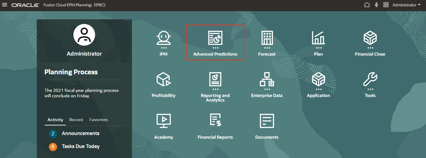
- Click Advanced Predictions.

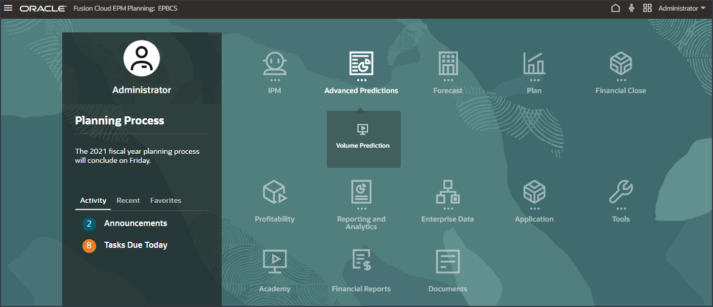
This is a navigation flow where you can review the predictions generated using Advanced Predictions.
Reviewing Volume Predictions
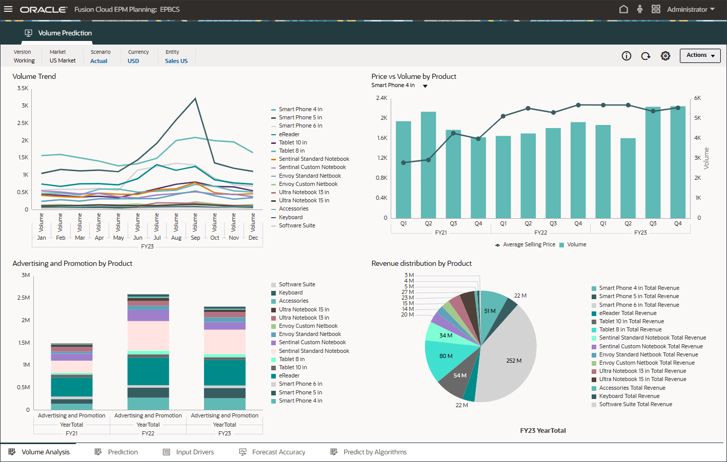
Before creating and running volume predictions, you review the volume predictions dashboard along with historical data that has been prepared for this use case. You use the Volume Predictions card that is set up to show analysis of volume by period and other drivers. This card also includes tabs that are set up to show the driver values and the prediction results.
- On the home page, click Advanced Predictions, and then Volume Prediction.
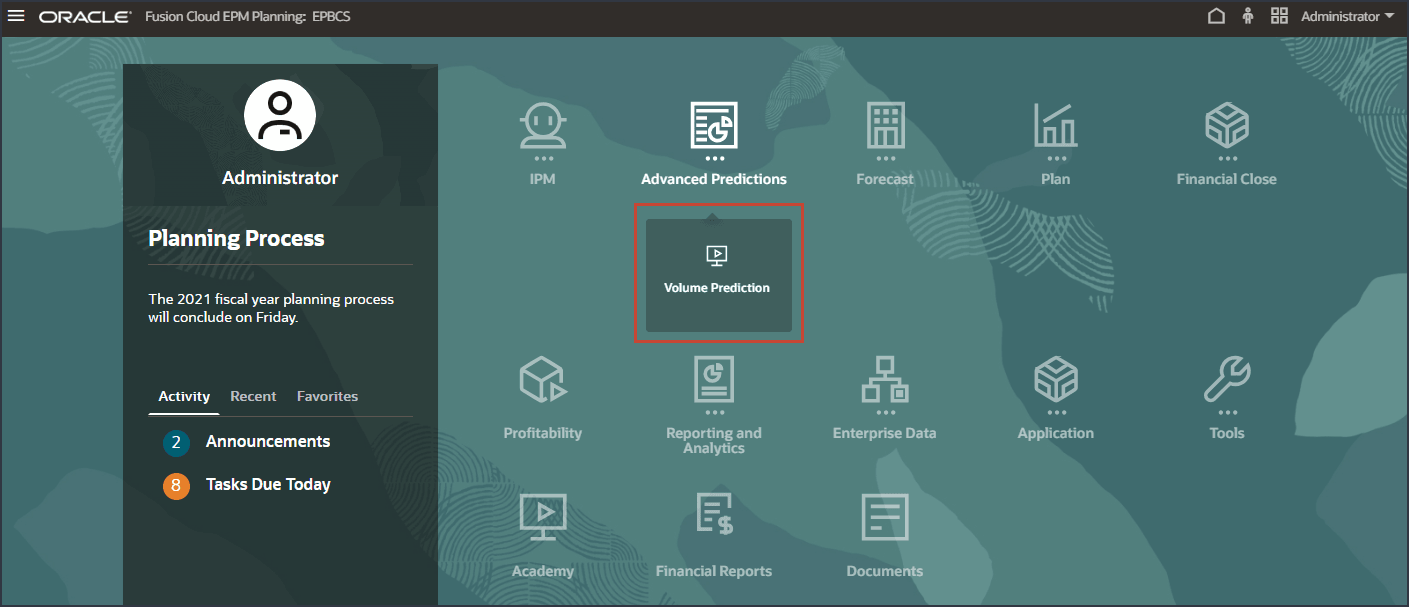
- Review volume predictions including Volume Trend, Price vs Volume by Product, Advertising and Promotion by Product, and Revenue distribution by Product.
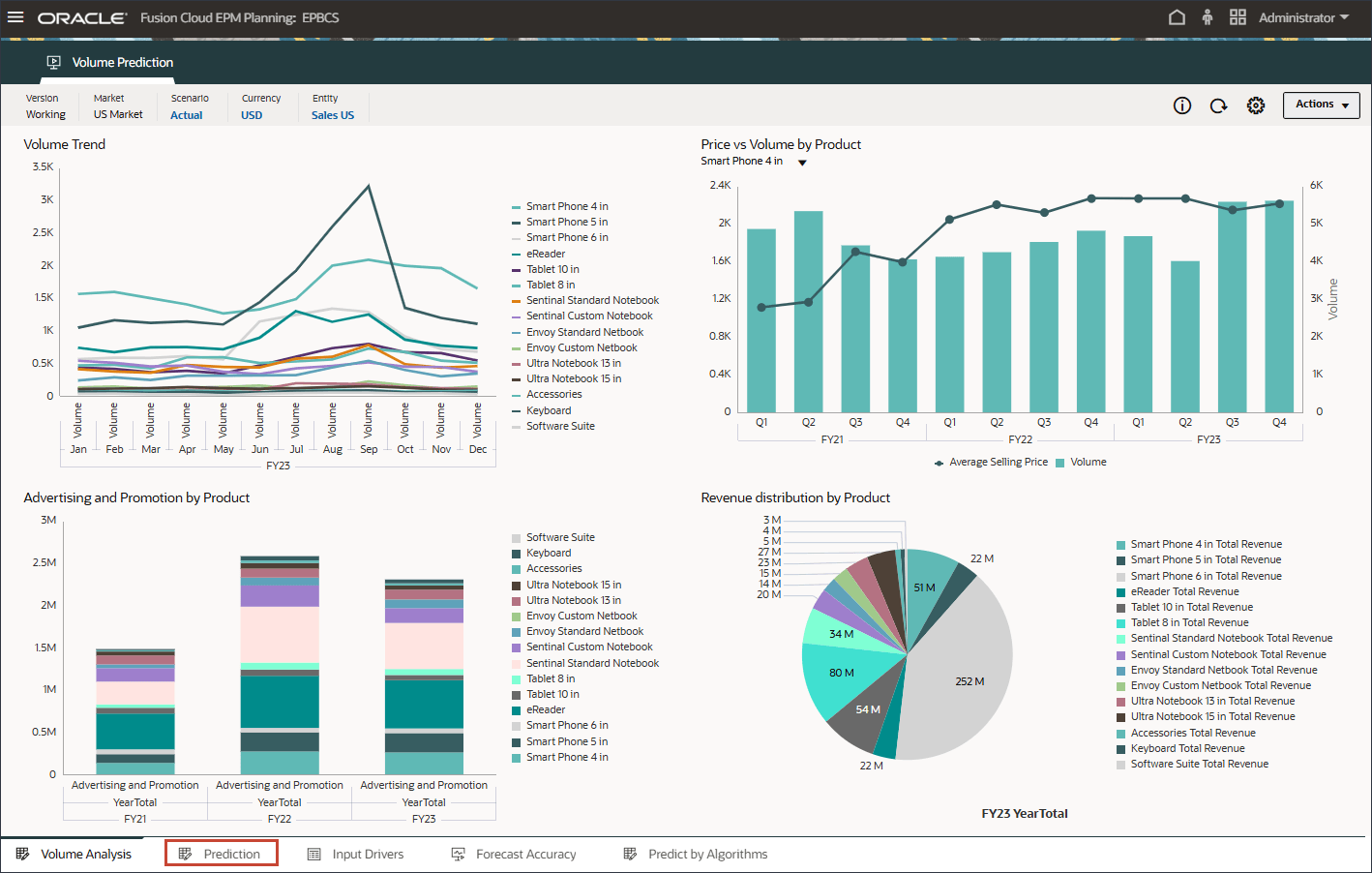
- On the bottom, click the Prediction tab.
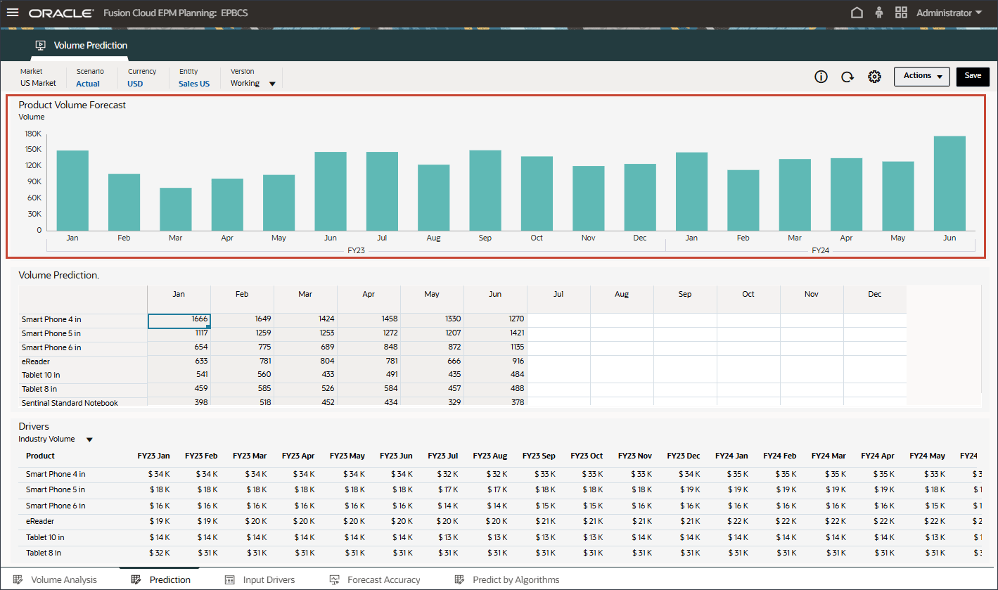
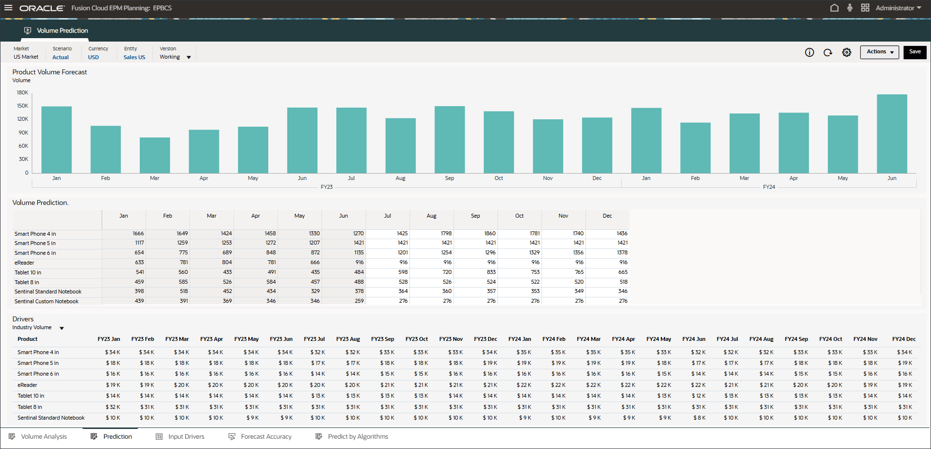
- In the bar chart on the top, review the historical volume forecast.
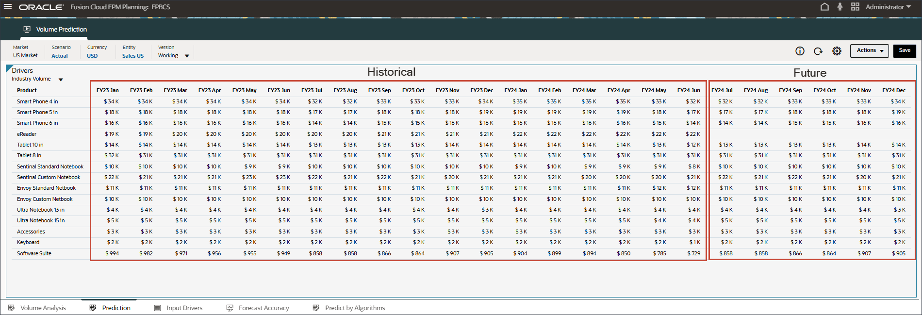
- In the Drivers grid on the bottom, review the driver data used in advanced predictions. This includes both historical and future driver data.
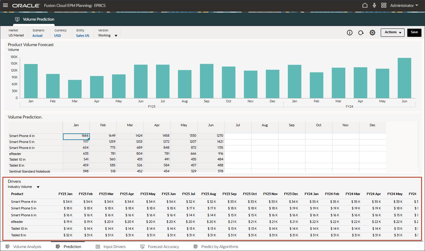
While the historical actual data for drivers can be sourced from different systems through integration, future driver data can be either derived through traditional forecast methods such as driver / trend / manual based or it can be based on a setting in the Advanced Prediction job to generate input driver data automatically using univariate prediction (statistical methods).
- In Drivers, click Industry Volume to review the drivers. Then after reviewing drivers, click Industry Volume again to close the list.
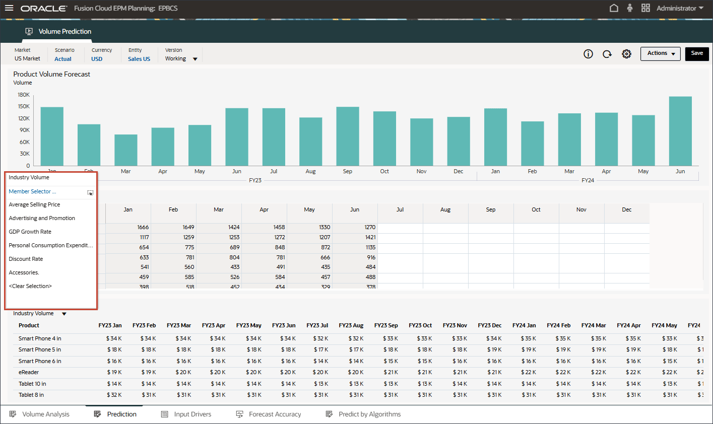
You can select one of several drivers including Average Selling Price, Advertising and Promotion, and Discount Rate.
- In the Drivers grid, click
 (Actions), and select Maximize.

- Review input drivers for both past and future data for Industry Volume.
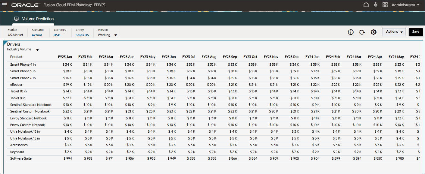
- Scroll to the right, to review future values.
- In the Drivers drop-down, click Industry Volume and select Average Selling Price.
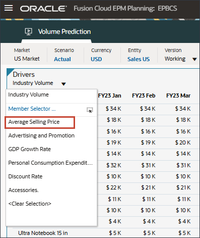
Data for the average selling price is displayed.
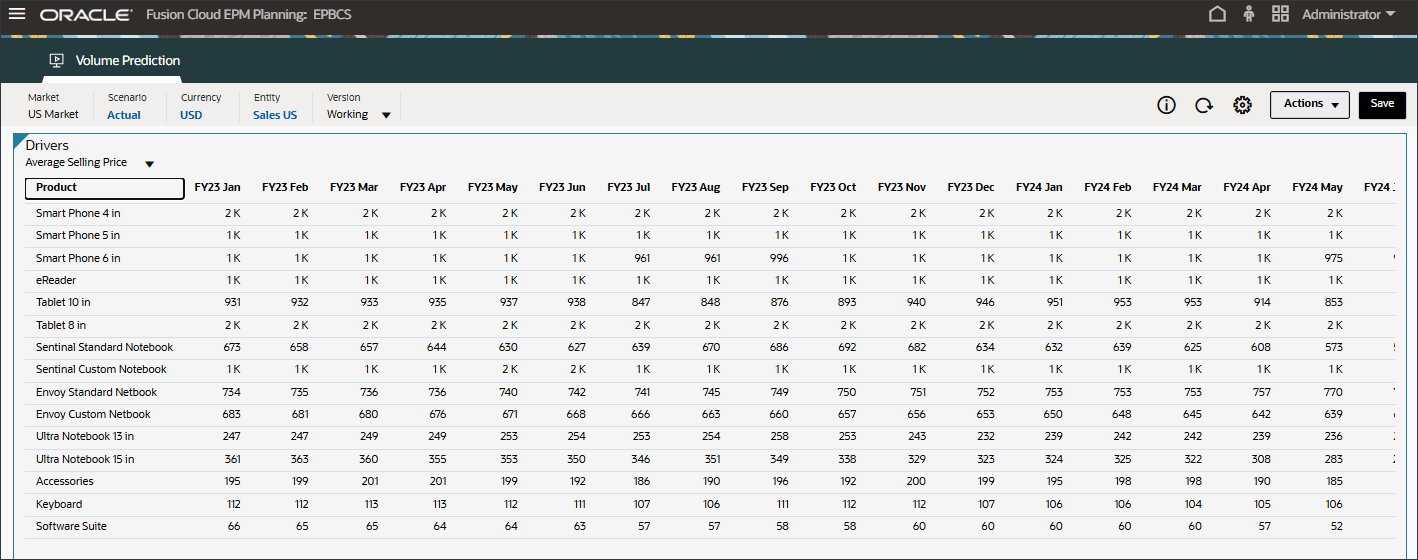
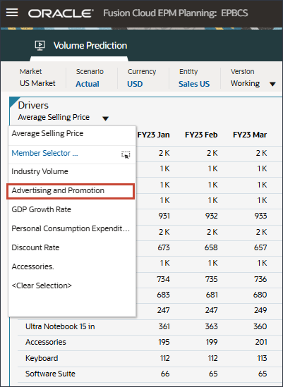
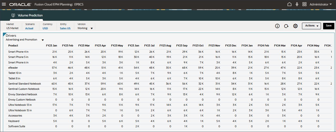
- In the Drivers drop-down, click Average Selling Price and select Advertising and Promotion.
Data for advertising and promotion is displayed.
- In the Drivers drop-down, click Advertising and Promotion and select GDP Growth Rate.
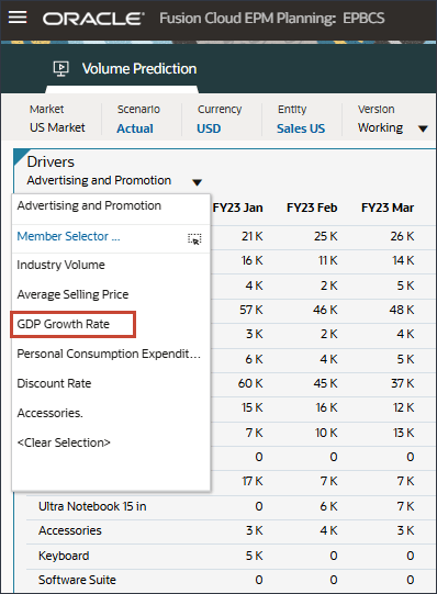
Data for GDP Growth Rate is displayed.
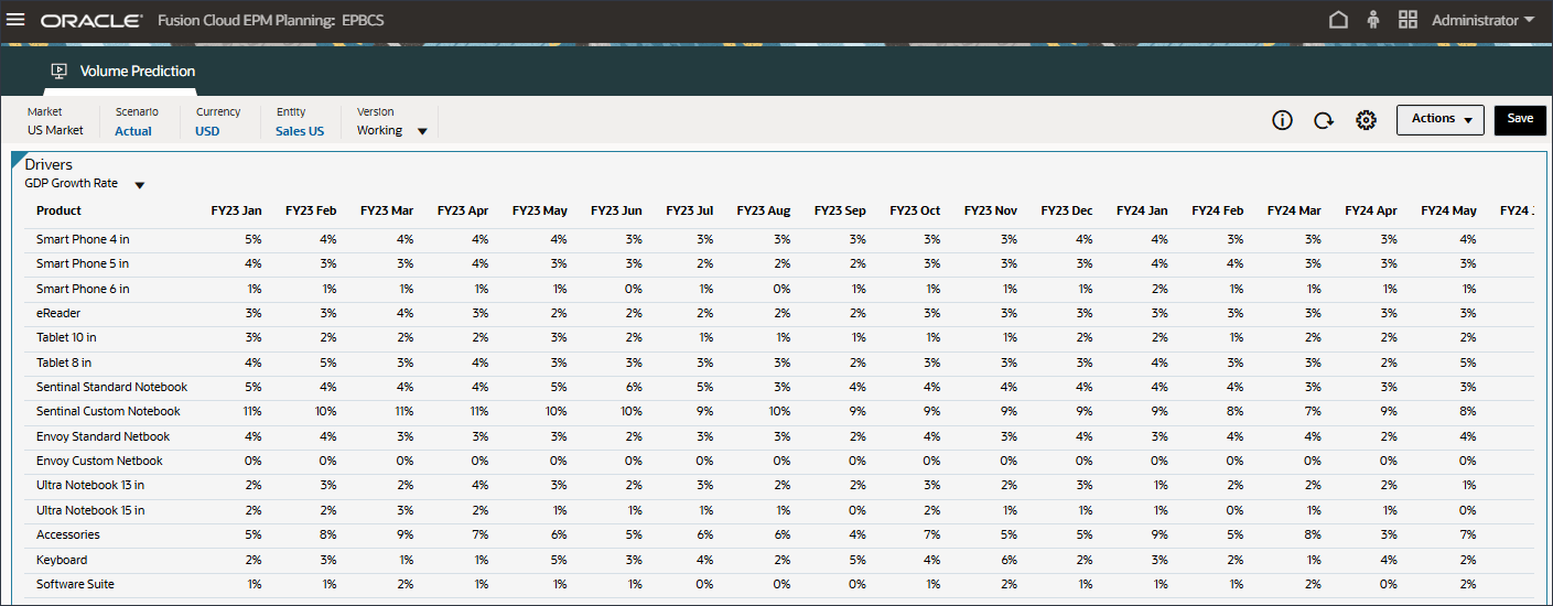
- In the Drivers drop-down, click GDP Growth Rate and select Personal Consumption Expenditure (Durable Goods).
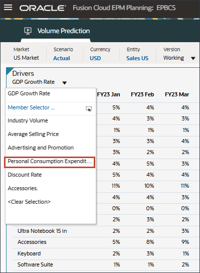
Data for Personal Consumption Expenditure (Durable Goods) is displayed.
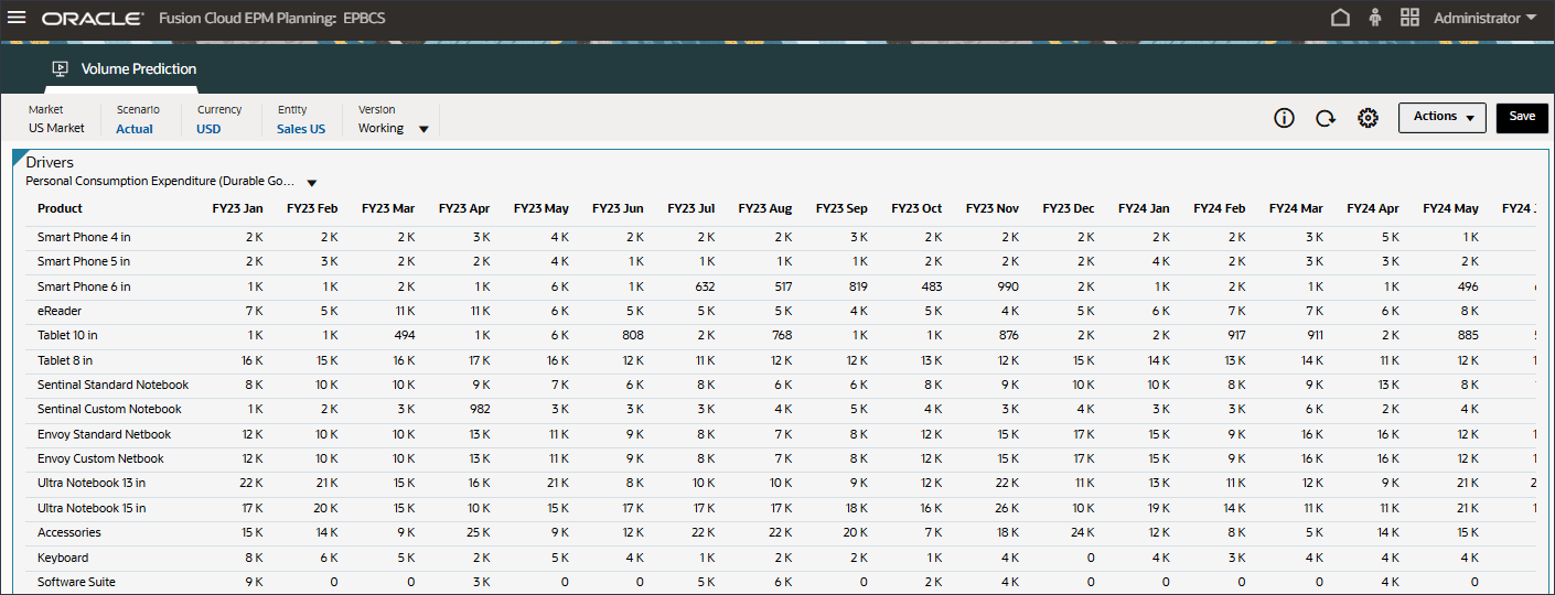
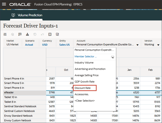
- In the Drivers drop-down, click Personal Consumption Expenditure (Durable Goods) and select Discount Rate.
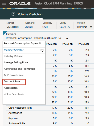
Data for Discount Rate is displayed.
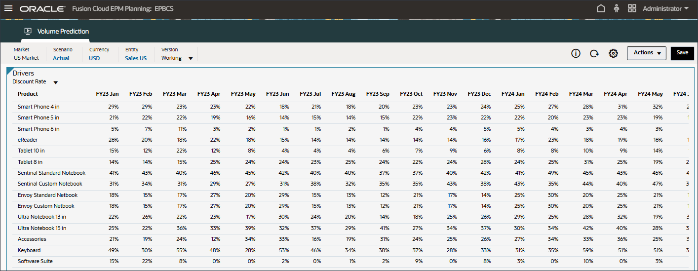
- On the bottom of the page, click the Input Drivers tab.
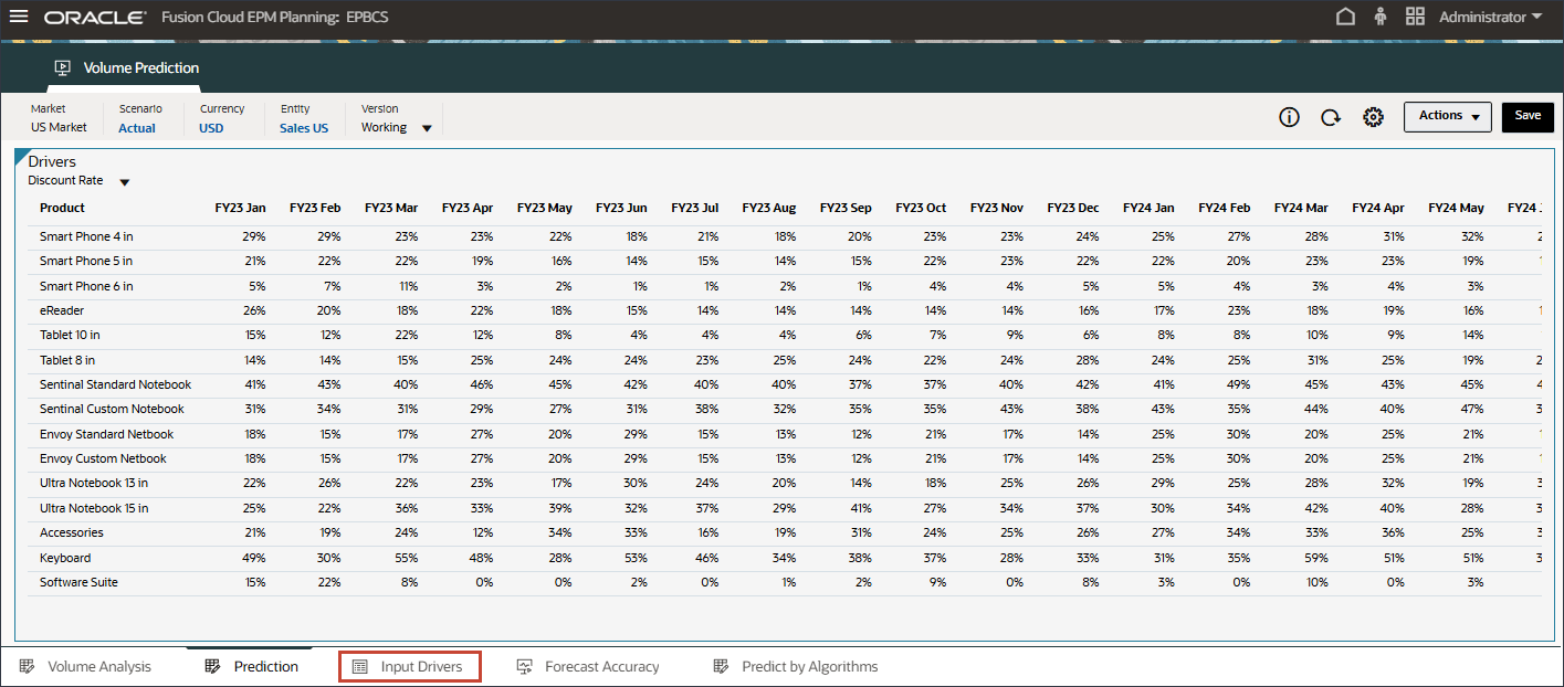
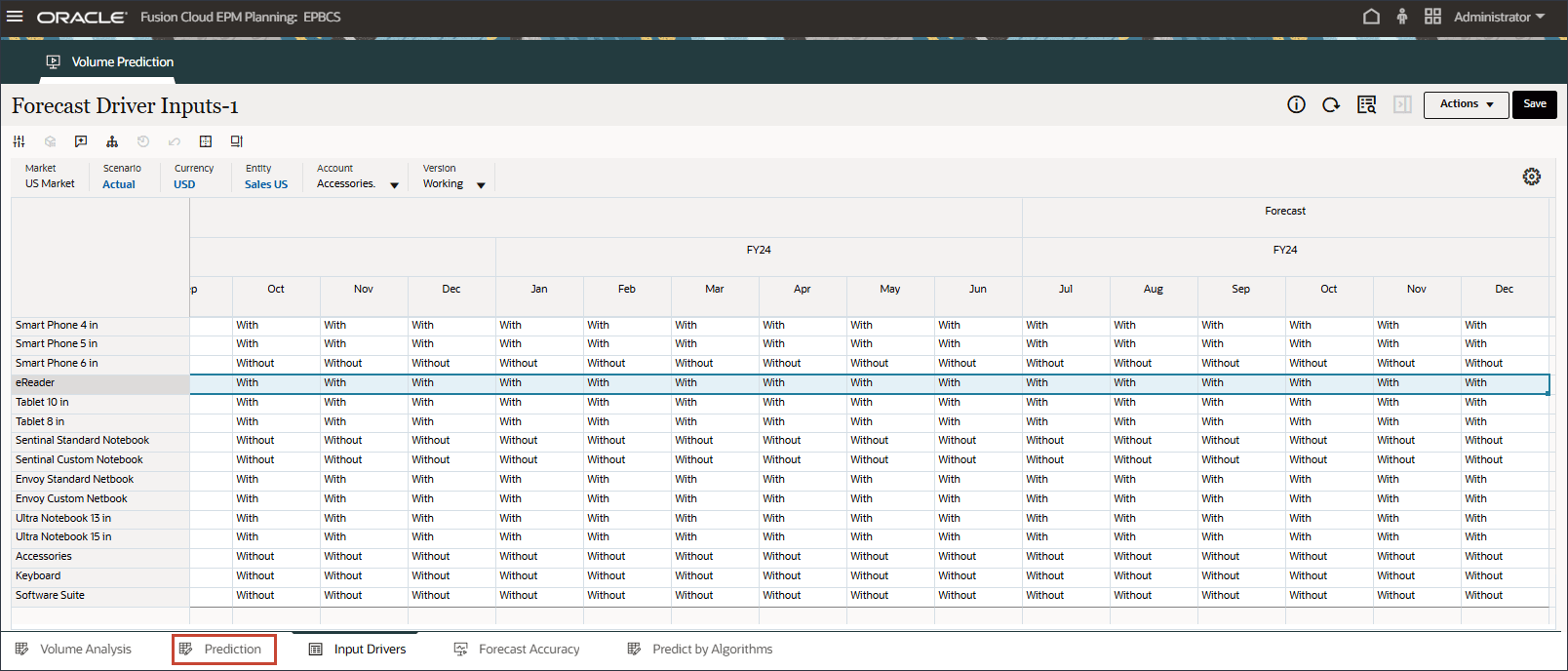
The Forecast Driver Input is displayed.
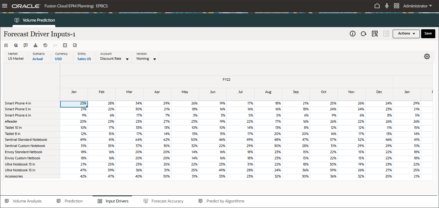
- In Account, click Discount Rate, and select Industry Volume.
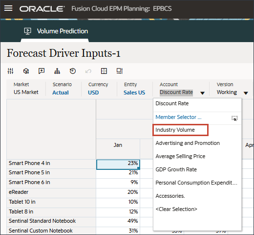
If you made changes, click Save to save the changes.
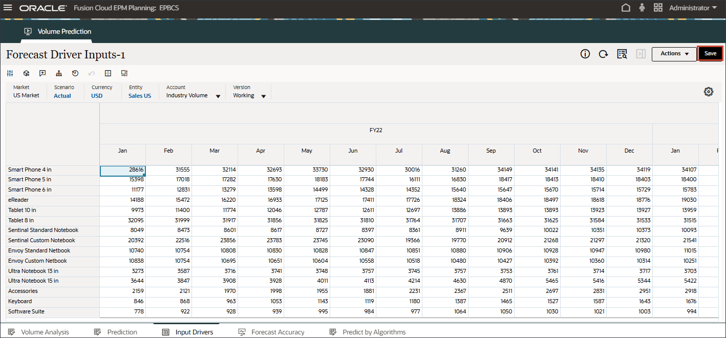
Similarly, you can select any driver and edit it.
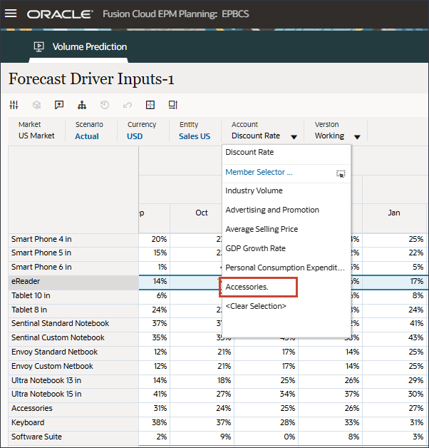
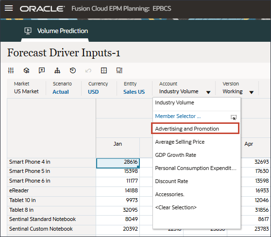
- In Account, click Industry Volume, and select Accessories.
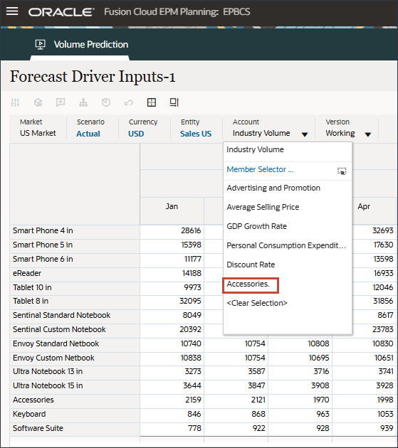
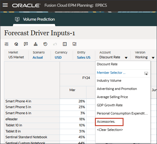
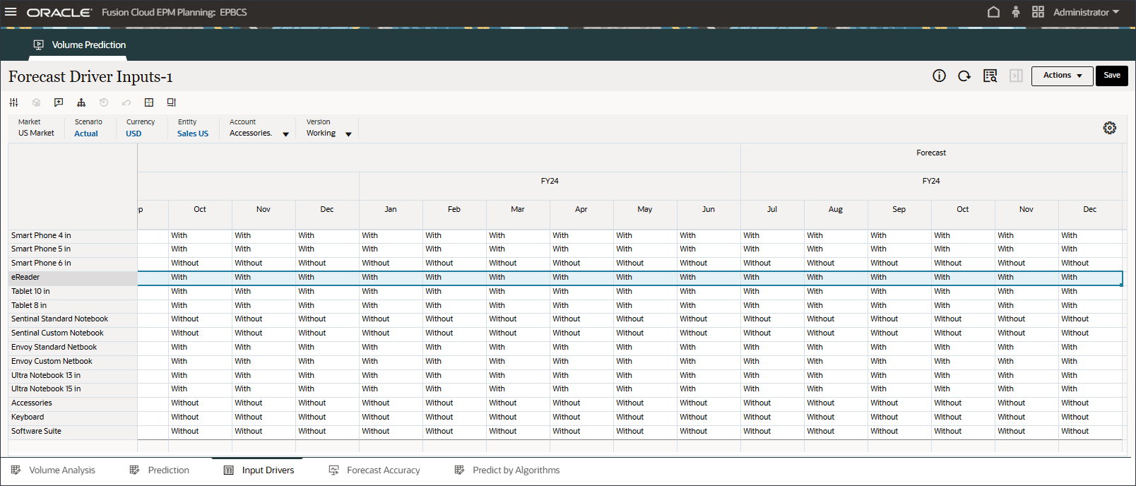
The Accessories driver uses a smart list. In Data Science this is referred to as categorical variables. To calculate future sales volume, you can use a numeric value or a smart list value. In this case, depending on the selected smart list value (with or without accessories), future sales volume predictions can be impacted.
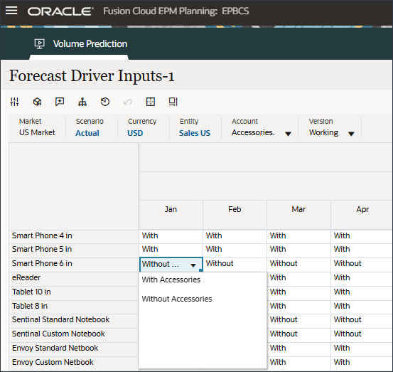
- In Account, click Accessories, and select Industry Volume.
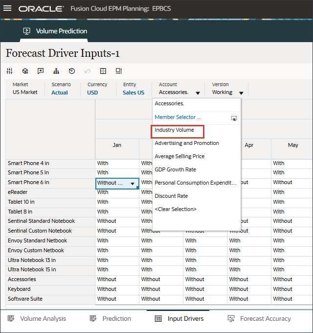
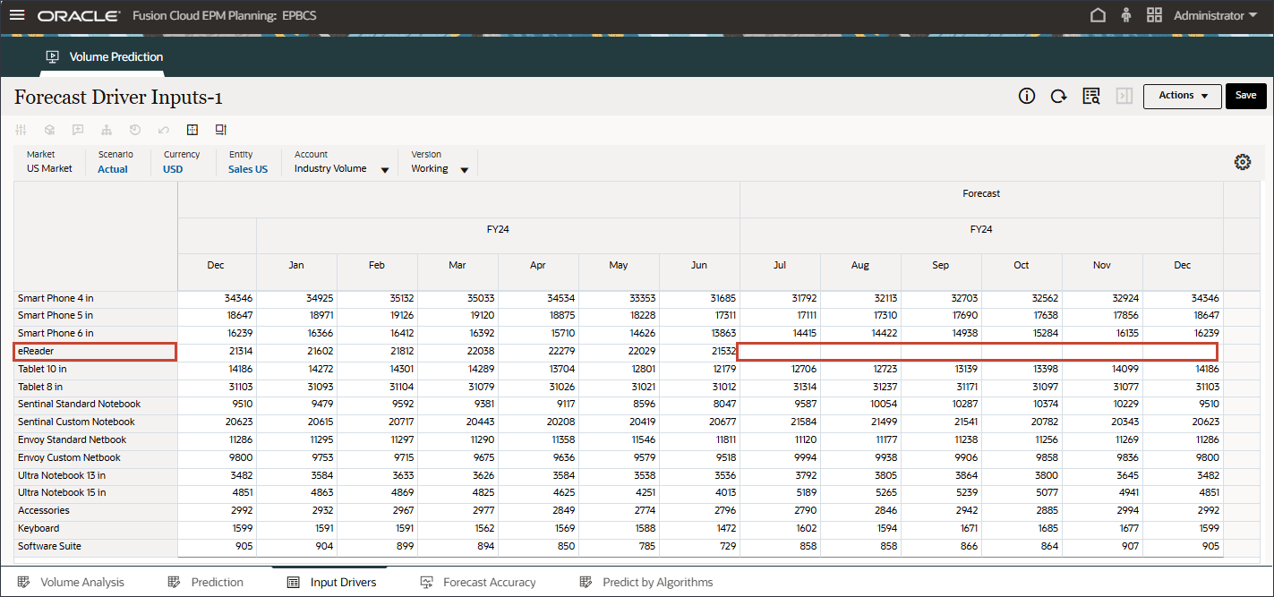
- Scroll to the right, and for eReader, for Forecast, notice the missing values for industry volume between July and December FY24.
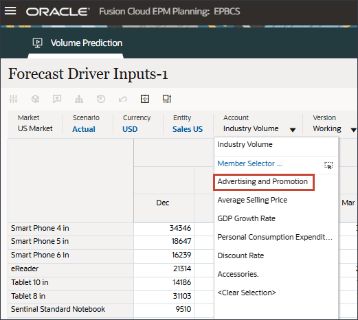
- In Account, click Industry Volume, and select Advertising and Promotion.
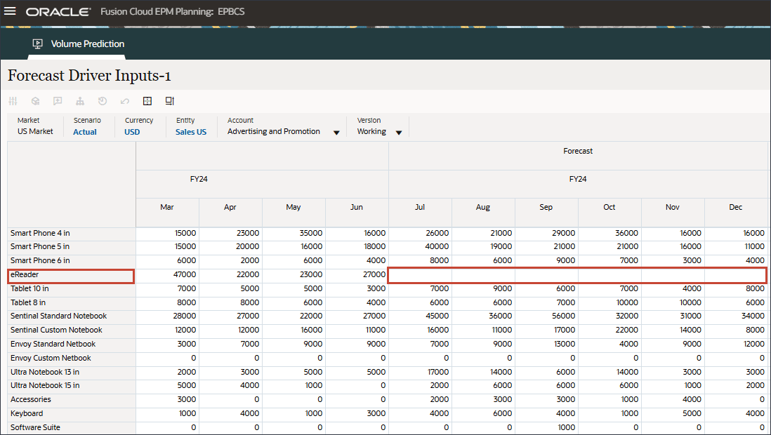
- Scroll to the right, and for eReader, for Forecast, notice the missing values for Advertising and Promotion between July and December FY24.
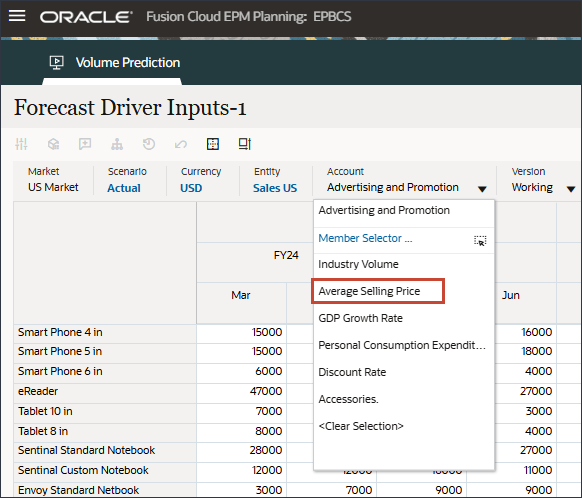
- In Account, click Advertising and Promotion, and select Average Selling Price.
- Scroll to the right, and for eReader, for Forecast, notice the missing values for Average Selling Price between July and December FY24.
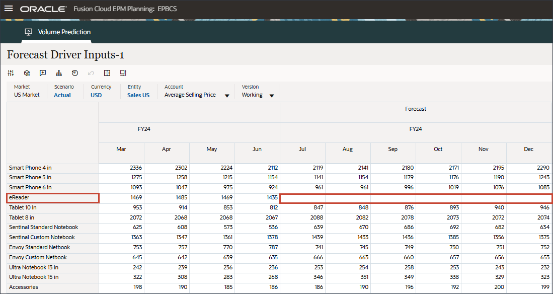
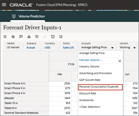
- In Account, click Average Selling Price, and select Personal Consumption Expenditure (Durable Goods).
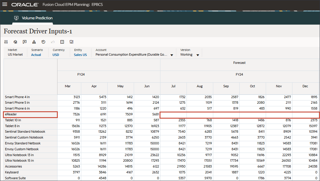
- Scroll to the right, and for eReader, for Forecast, notice the missing values for Personal Consumption Expenditure (Durable Goods) between July and December FY24.
- In Account, click Personal Consumption Expenditure (Durable Goods), and select Discount Rate.
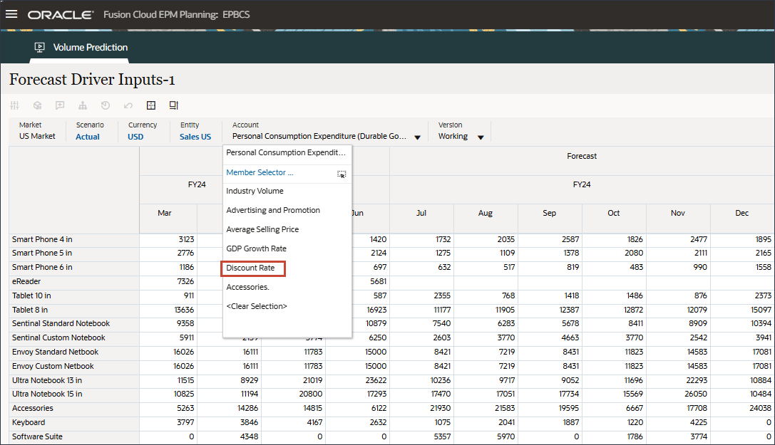
- Scroll to the right, and for eReader, for Forecast, notice the missing values for Discount Rate between July and December FY24.
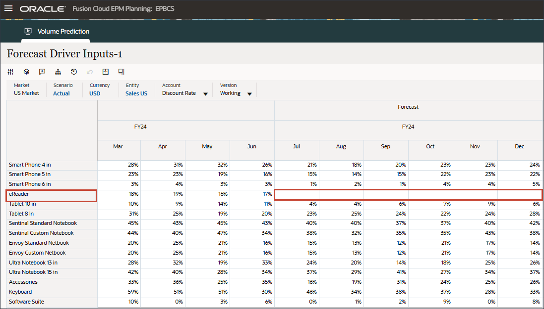
- In Account, click Discount Rate, and select Accessories.
- Scroll to the right, and for eReader, for Forecast, notice the missing values for Accessories between July and December FY24.
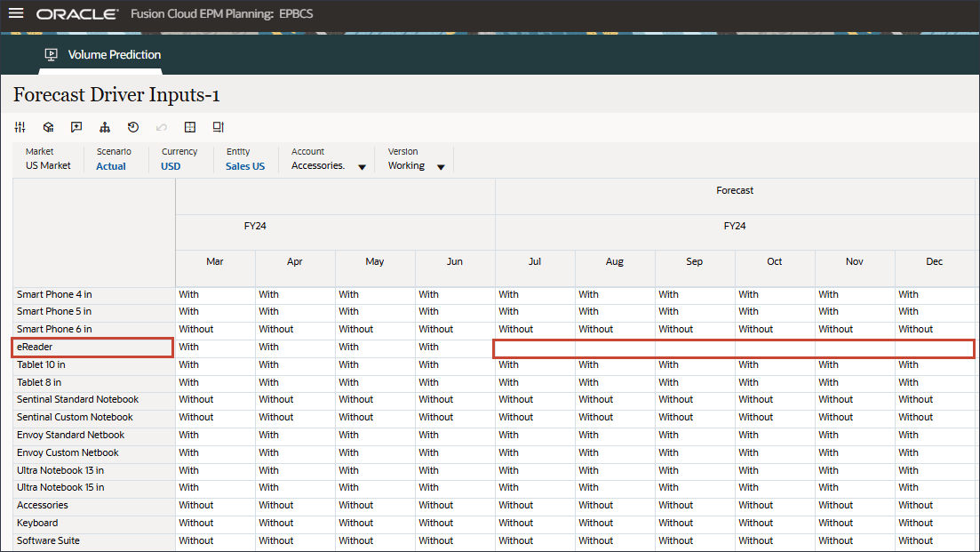
Advanced Predictions can predict missing input driver values. In a later section of this tutorial, you will configure the Advanced Prediction job to ensure that the future input driver values for eReader are predicted.
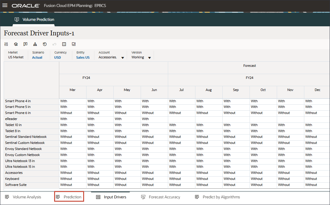
- On the bottom, click the Prediction tab.
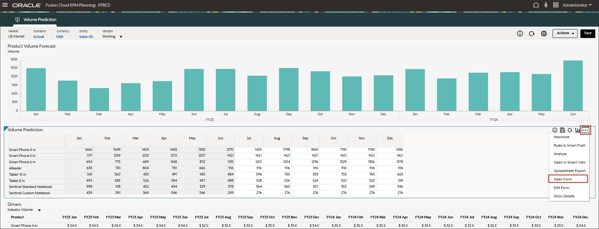
- On the Volume Prediction form, on the right, click
 (Actions), and select Open Form.
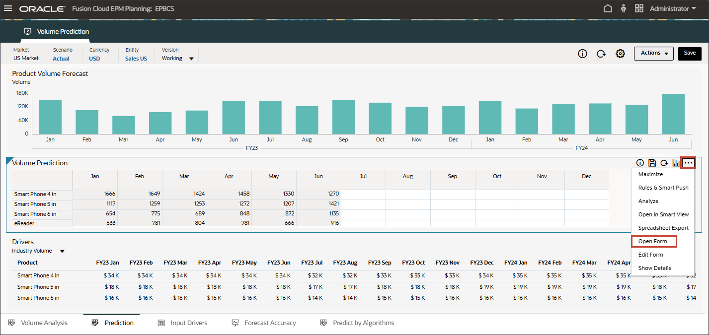
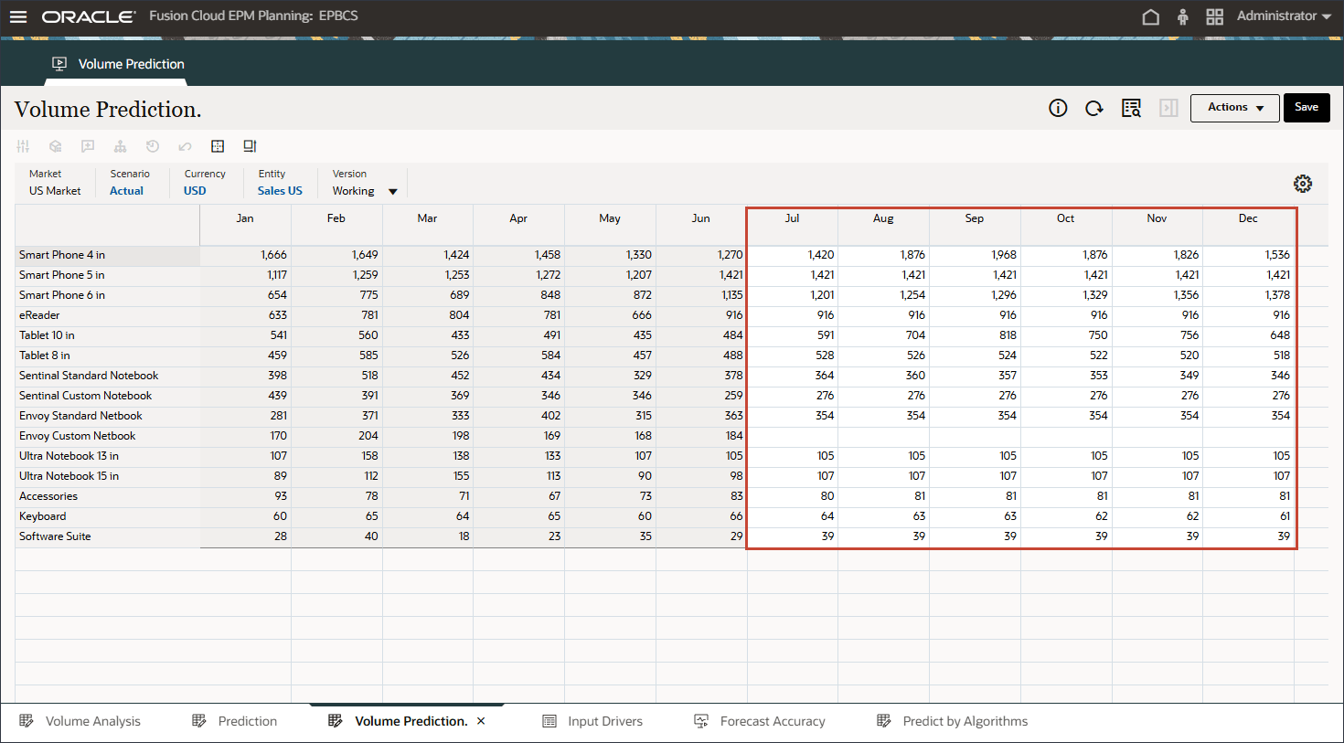
- Notice that the prediction results are missing for periods July to December FY24.
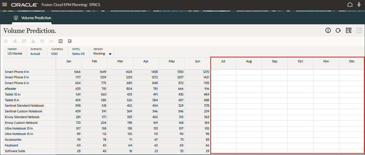
These are the periods we would like to predict for all the products using the advanced predictions capability.
- Click
 (Home) to return to the Home page.
The Prediction tab shows the dashboard with the volume that is planned to be predicted and it also contains the table with all the drivers that will be used to predict volume.
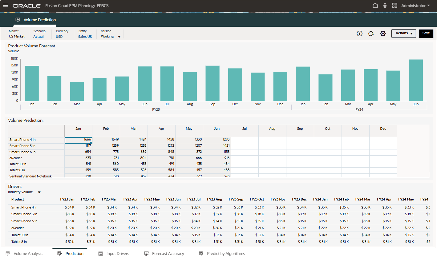
These input drivers are instrumental for deriving the volume prediction accurately with advanced prediction Algorithms.
Editing Input Drivers
You can edit any of the input drivers. You can edit both historical and future data.
Reviewing Missing Input Driver Values for Future Periods
In this section, you check for missing input drivers.
Reviewing the Predictions Form
In this section, you review the Volume Prediction form for missing values.
Configuring Advanced Predictions
In this section, you configure Advanced Predictions to predict future product volumes.
You complete the steps in the IPM Configuration wizard to configure Advanced Predictions.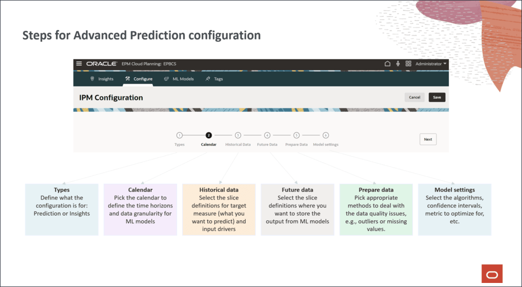
Setting up the Advanced Predictions Calendar
Before you can configure Advanced Predictions, you must define a calendar that includes both historical and future periods.
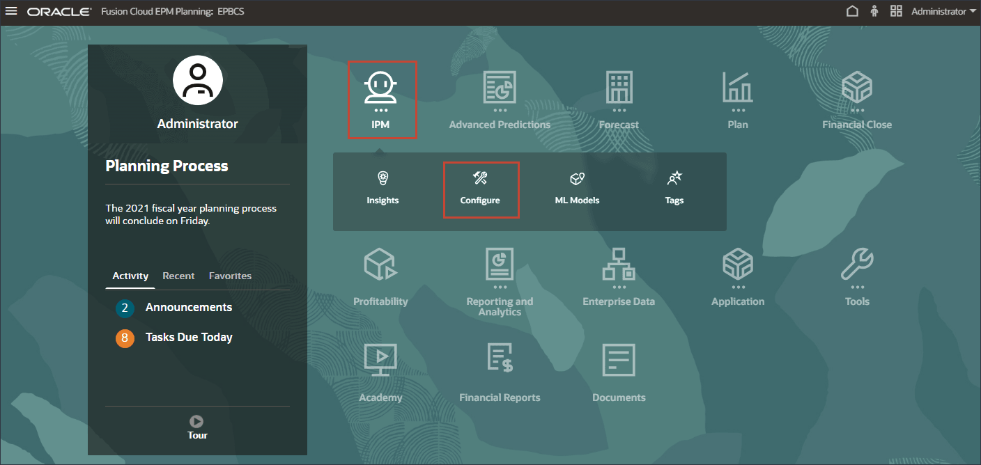
- On the home page, click IPM then Configure.
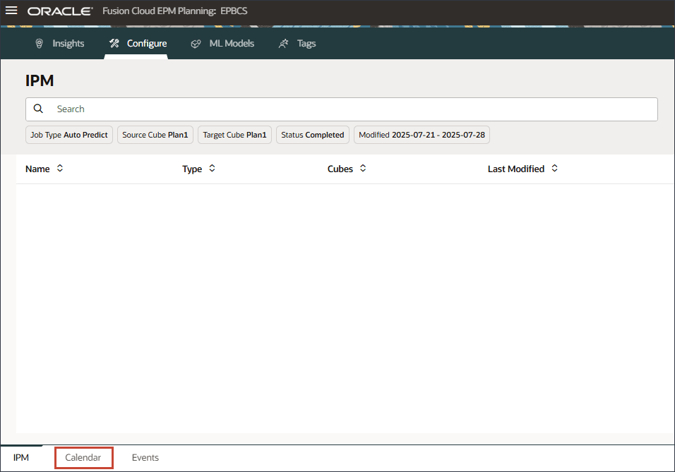
- On the bottom, click the Calendar tab.
- Click Add Calendar.

- In Name and Description, enter Volumeforecast-Monthly.
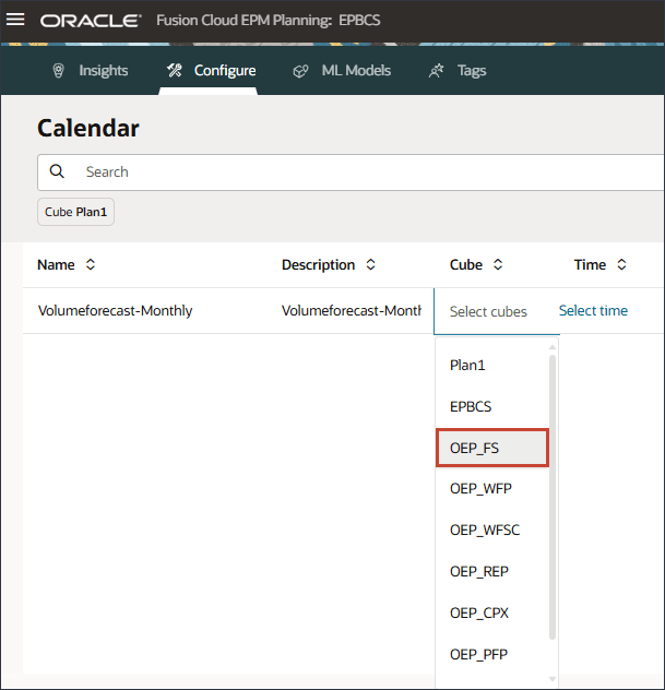
- For Cube, select OEP_FS.
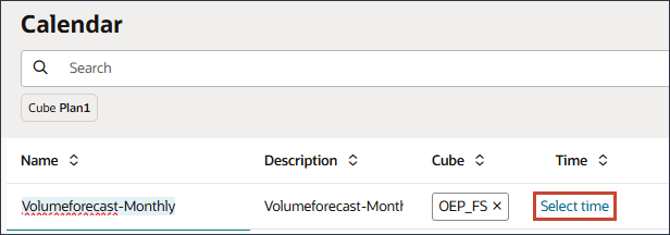
- For time, click Select time.
- In Select Members, for Years, for All Year, and select FY22, FY23, and FY24.

For time you include the entire range of historical and future periods required for predictions.
- Click Period.

- For YearTotal, select
 (Function Selector), and select Level 0 Descendants.

The selection is displayed.

For the period, you can include the historical period from when you want to use the data. For the future you want to predict, you can include as many years for future data for which you would like to predict. In this example, you selected years – FY22, FY23, and FY24 and periods – all level 0 descendants of YearTotal (all months).
- Click OK.
The year and period selections are included in the calendar.
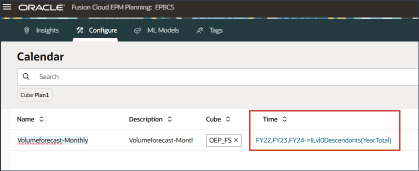
- Click Select current date.

- For Years, select FY24.
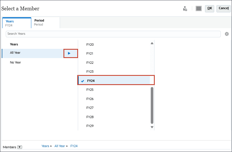
- Click Period.
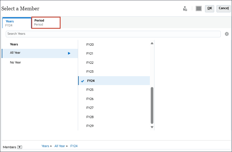
- Under YearTotal, and Q3, select Jul, and click OK.
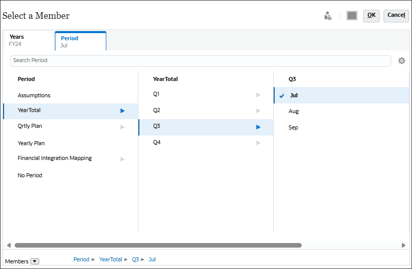
Note:
You can set current year by using substitution variables. - For Number of Historical periods, enter 30, and for Number of Future periods, enter 6.

- Click
 (Save).
 - For Volumeforecast-Monthly, click
 (Actions), and select Edit.

- Click
 (Date Mapping).
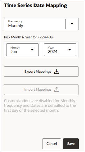
Date mapping which defines the frequency and date format is an important step to send the period data to the data science engine.
- For Month, select July and for Year select 2024, and click Save.

- To review the mappings, for the VolumeForecast-Monthly calendar, click
 (Actions), and select Edit.

- Click
 (Date Mapping).
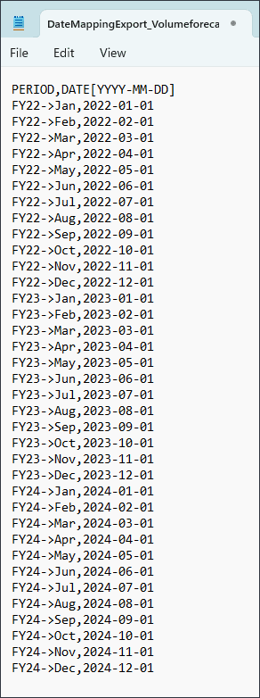
 - Click Export Mappings.
You can open the file and review the mappings. Be sure to open the .csv file with Notepad.
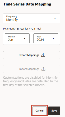
- Close the Notepad file, and in Time Series Date Mapping, click Cancel.
Caution:
Ensure that you save the calendar before setting up the date mapping by clickingCreating Custom Calendars
Since GDP Growth Rate is stored at BegBalance for FY22, FY23, and FY24, you create a custom calendar so that Advanced Predictions can include the inputs from the BegBalance period.
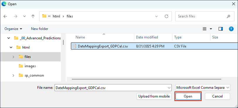
- Before you create a custom calendar, open the DateMappingExport_GDPCal.csv file in notepad to review its contents.

The file includes BegBalance for each year from FY22 to FY29 for the first day of July.
- Close Notepad.
- Click Add Calendar.

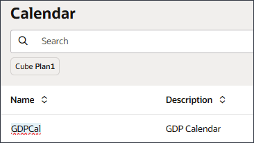
- In Name, enter GDPCal.
- In Description, enter GDP Calendar.
- For Cube, select OEP_FS.
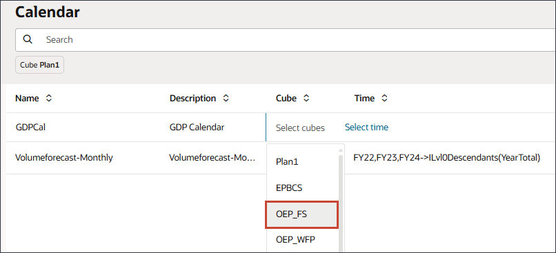
- For time, click Select time.
- In Select Members, for Years, for All Year, click
 (Function Selector), and select Level0Descendants.
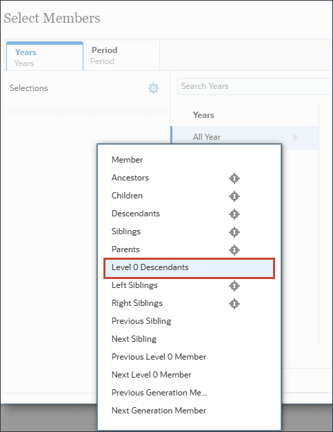
For time you include the entire range of historical and future periods required for predictions.
- Click Period.
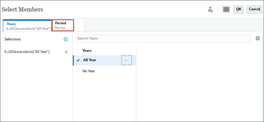
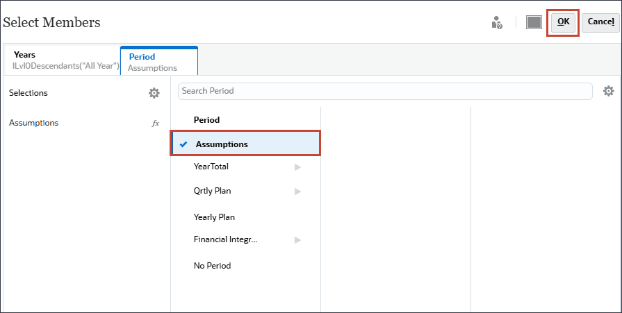
- For Period, select Assumptions, and click OK.
- Click Select current date.

- For current date, for Years, select FY24, and for Period, select Assumptions, and click OK.
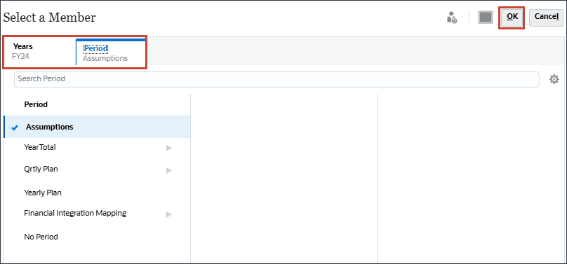
- For Number of Historical periods, enter 2, and for Number of Future period, enter 1, and then click
 (Save).

-
In the GDPCal row, click
 (Actions), and select Edit.

-
Click
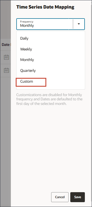
 (Date Mapping).
- In Date Mapping, for Frequency, select Custom.
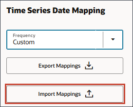
- Click Import Mappings.
- Locate and select DateMappingExport_GDPCal.csv, and click Open.
- Click Save.
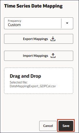
The Information message is displayed.

The GDP Calendar is added.

- Click
 (Home) to return to the Home page.
Caution:
Ensure that you save the GDPCal before setting up the date mapping by clickingConfiguring Advanced Predictions in IPM Jobs
- On the home page, click IPM, then Config.
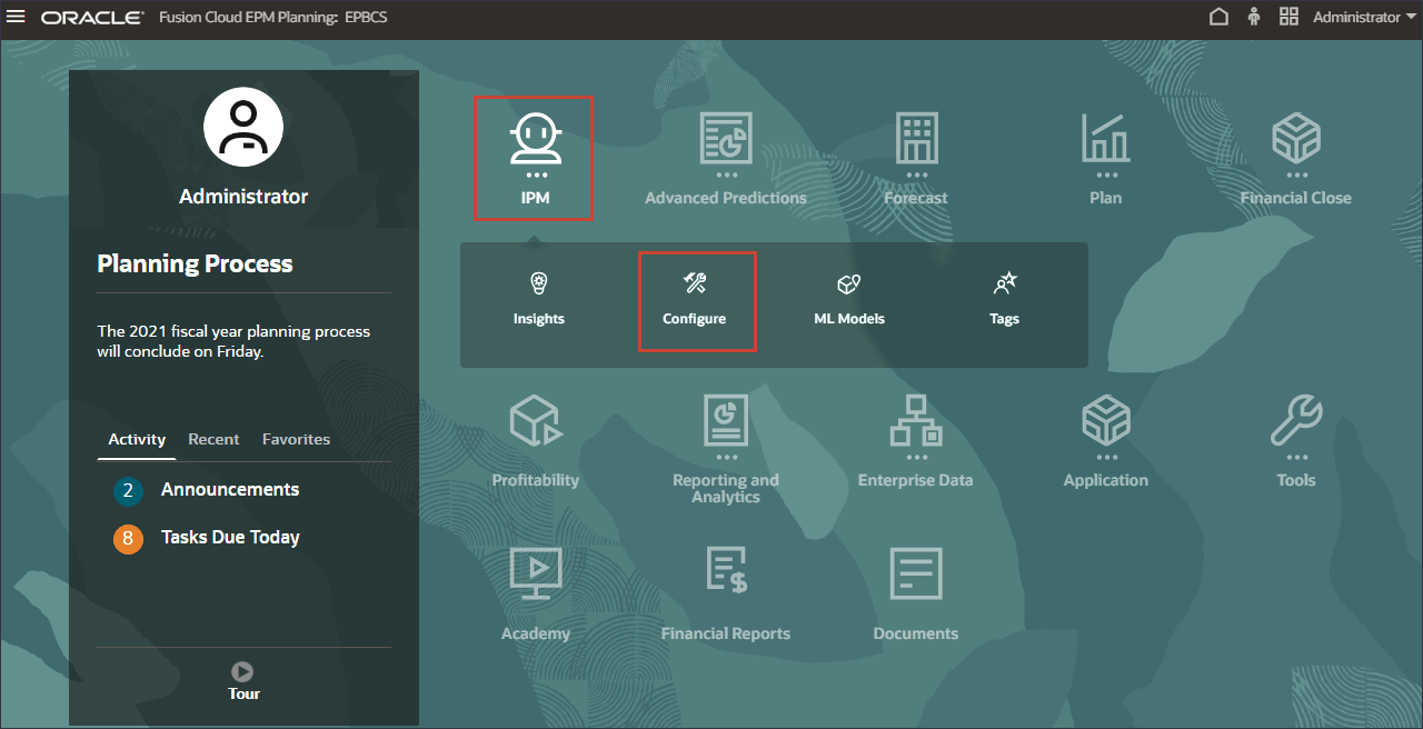
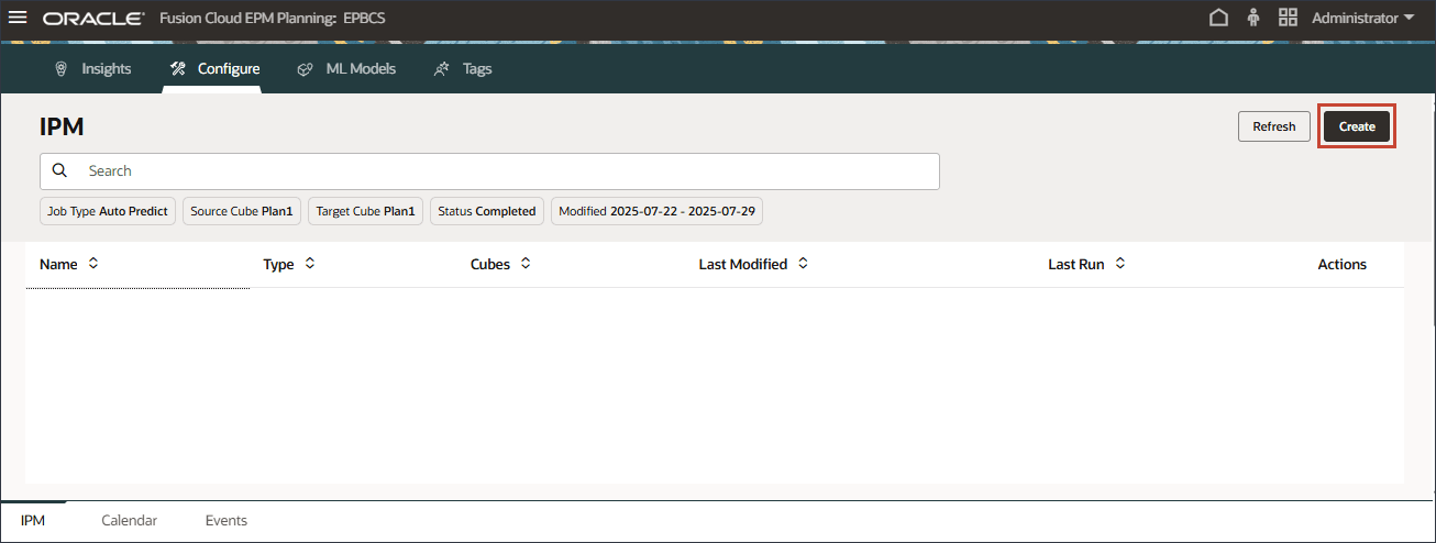
- Click the IPM tab.

- On the IPM page, click Create.
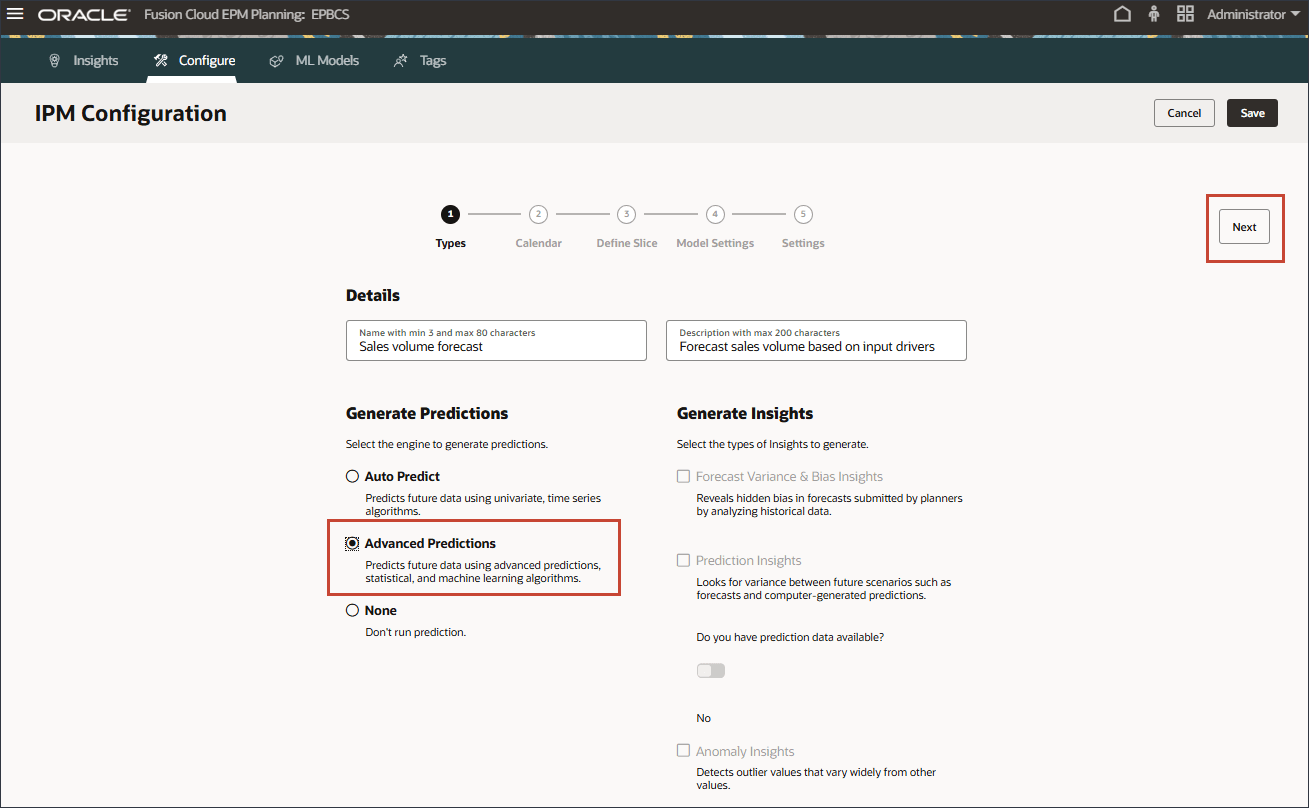
- In Details, for Name, enter Sales volume forecast, and for Description, enter Forecast sales volume based on input drivers.
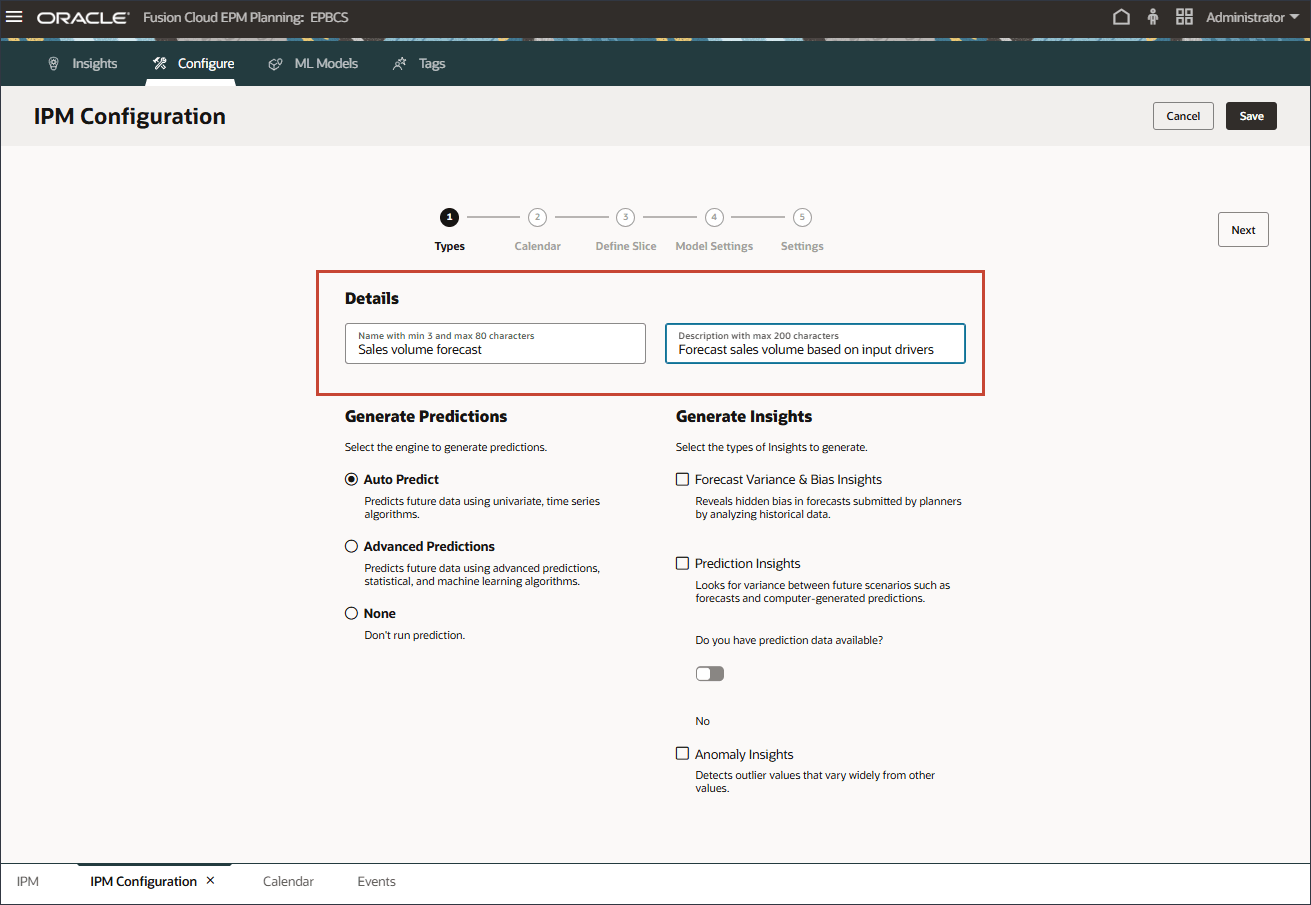
- To predict future data using multi-variate, statistical and machine learning algorithms, select Advanced Predictions, then click Next.
Picking the Calendar
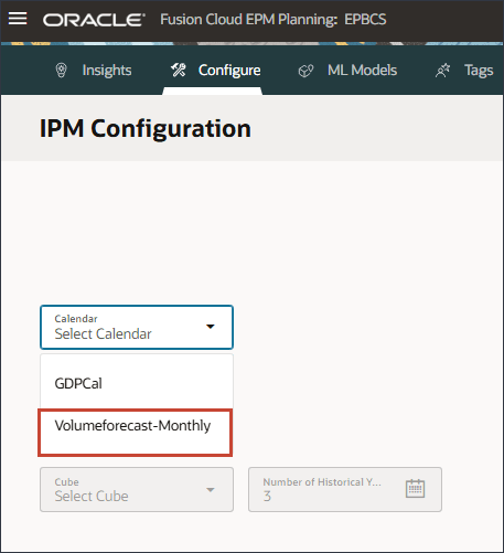
You can define the time range for historical and future periods either by selecting a calendar or manually providing the period range.
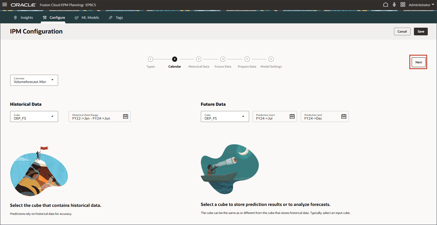
- To select a calendar, click Calendar, and select Volumeforecast-Monthly.
After selecting a calendar, the historical and future period ranges get filled in automatically.
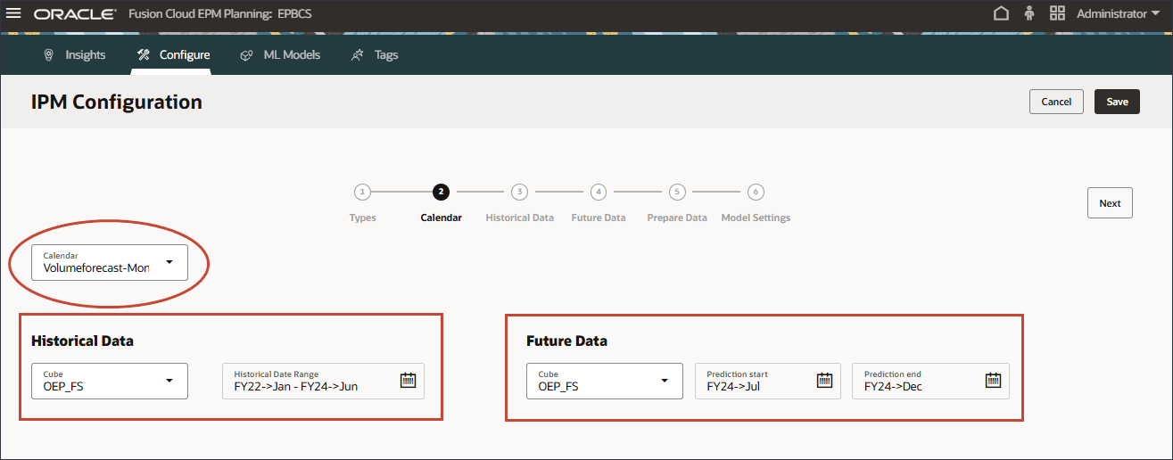
The cube selection is automatically filled in from the Calendar definition.
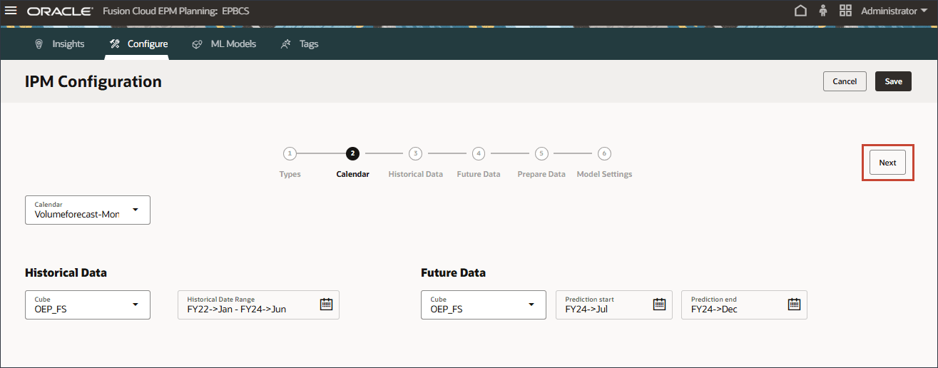
If you selected a calendar, then you cannot change the period range because the period range definition is populated from the calendar definition. If you want to make any changes to the period, you need to go back to the calendar setup and make the changes there.
- Click Next.
Note:
For Advanced Predictions, you cannot manually select historical data or future data in IPM Configuration. It is mandatory to predefine a calendar.Selecting the Slice Definition for Historical Data
In this section, you define what you want to predict, and the input drivers you want to use. You define the input drivers and map them to data in your cube. You must have those output measures and input drivers already defined in your EPM cube. As you reviewed earlier in the tutorial, you have the necessary account members and data for the various accounts – both the target and the input drivers.
In this configuration, the Account dimension contains the necessary measure and accounts for both output and input drivers so the Account dimension needs to be included in the rows of the configuration definition.
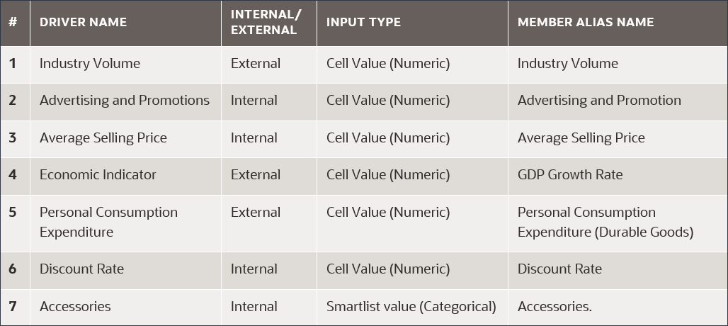
You define input drivers which are factors that are used to train the prediction model to predict the selected measure. There are seven input drivers:
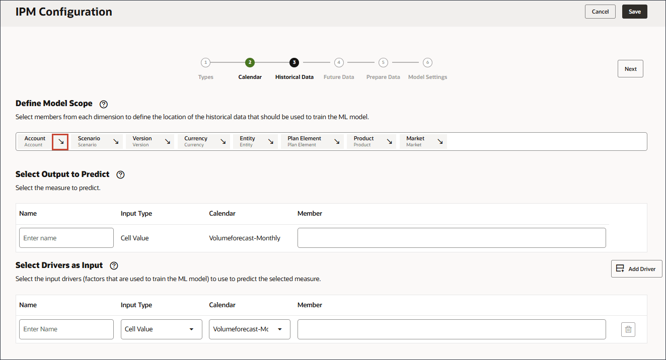
- To the right of Account, click the arrow.
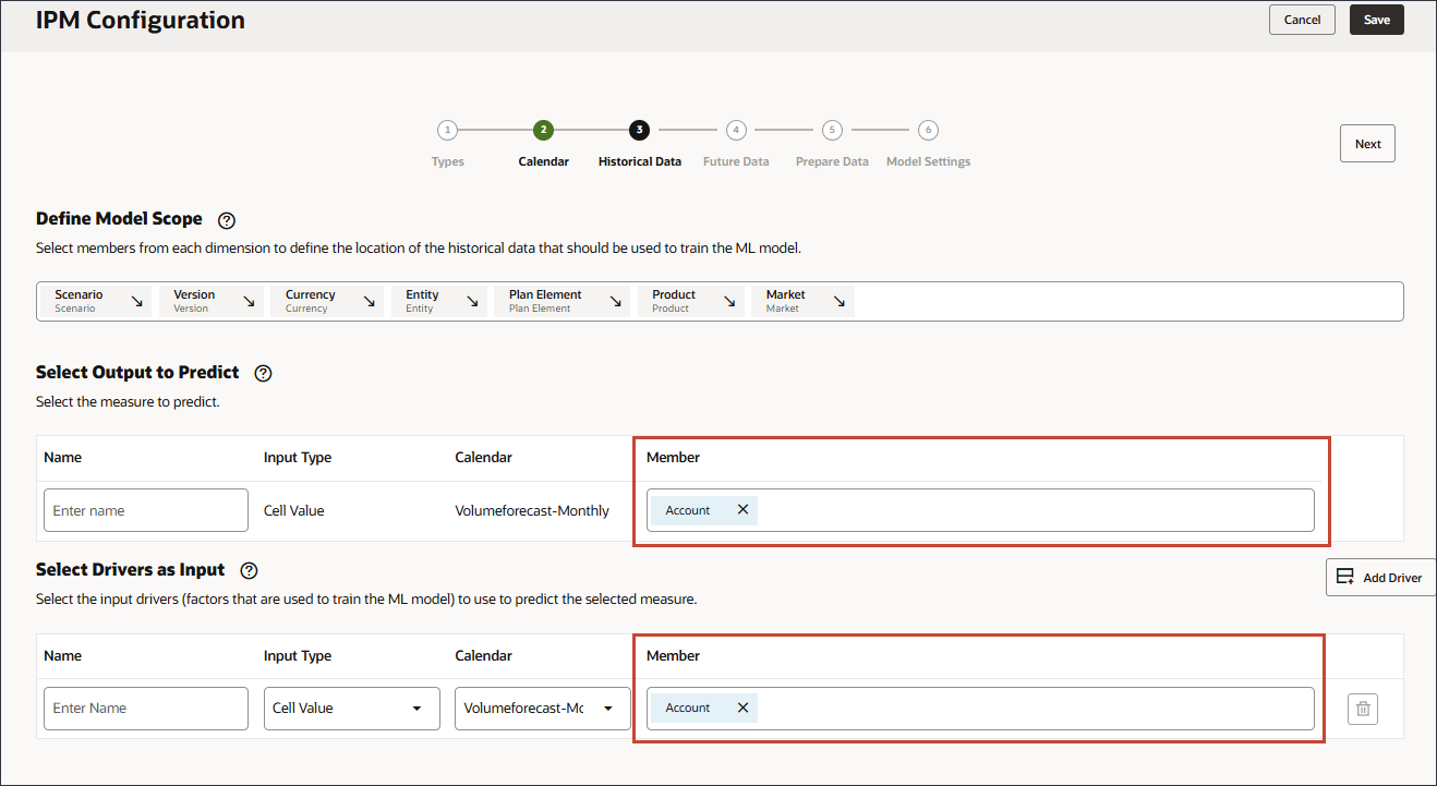
Account is added to the rows.
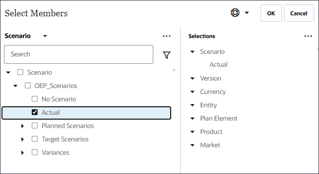
- For Scenario, click Scenario to open the Member Selector.

- Expand OEP_Scenarios, select Actual.
- Click Scenario, and select Version.
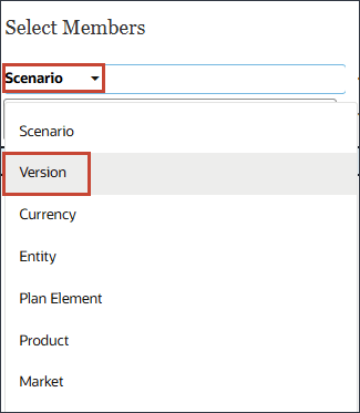
- Expand OEP_Versions, and select Working.
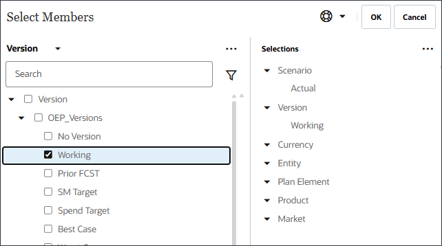
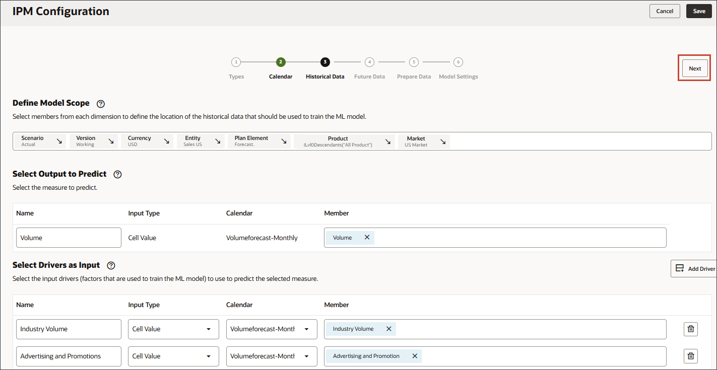
- Define the model scope by using Member Selector and selecting the following POV dimension members. After you selected all members, click OK.
Tip:
To define the POV (Model Scope), select each dimension and then select members including functions in the Select Members dialog. You can search for members.Dimension Member Scenario Actual Version Working Currency USD Entity Sales US Plan Element Forecast. Product Ilvl0Descendants(“All Product”) Market US Market Tip:
For Plan Element, you select "Forecast." which is under Plan Element, and Total Plan. "Forecast." is the alias for the OFS_Load member. The alias "Forecast." includes a period in the name.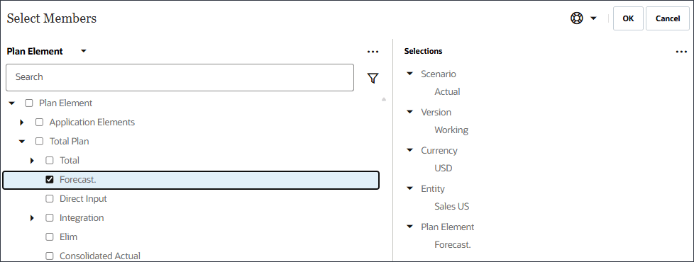
Tip:
For Product, you select Lev 0 Descendents of All Product.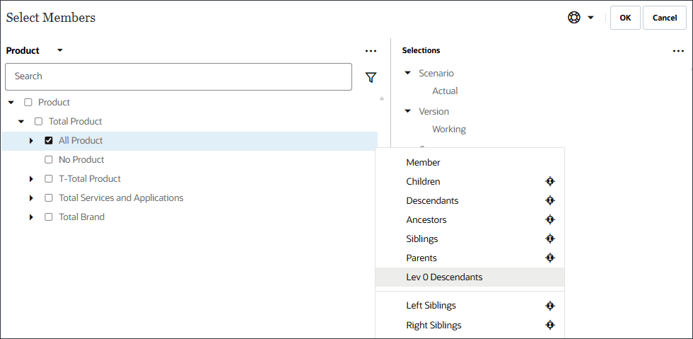
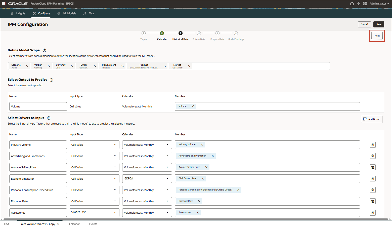
You select POV members from each dimension to define the location of the historical data that should be used to train the advanced prediction model. For example, train the advanced prediction model to predict volume for all members of Ilvl0Descendants("All Product"), use historical data from the Actual scenario and Working version, use USD currency, use the Sales US entity and so on.
- Verify your selections.

- In Select Output to Predict, for Name, enter Volume.
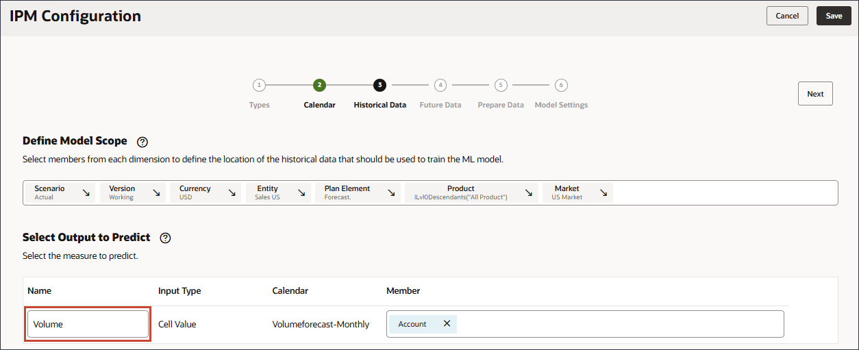
- In Select Output to Predict, click Account.
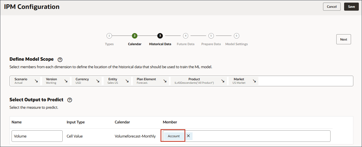
- Use Member Selector, to select Volume, and click OK.
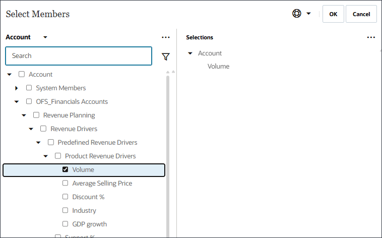
Caution:
Ensure you select the correct Volume account. The member name for this account is OFS_Volume while the alias is Volume.Volume is selected.
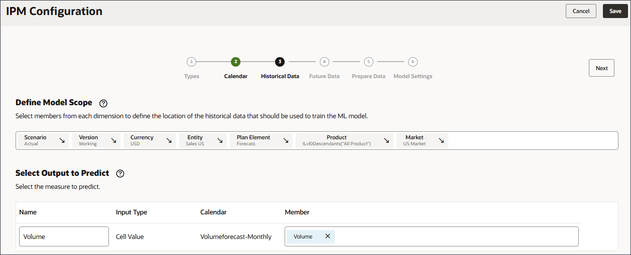
- In Select Drivers as Input, for Name, enter Industry Volume, and click Account.
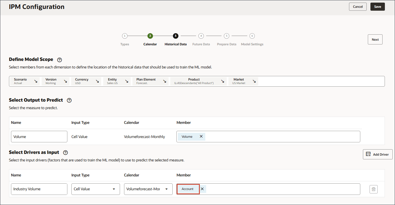
- Select Industry Volume, and click OK.
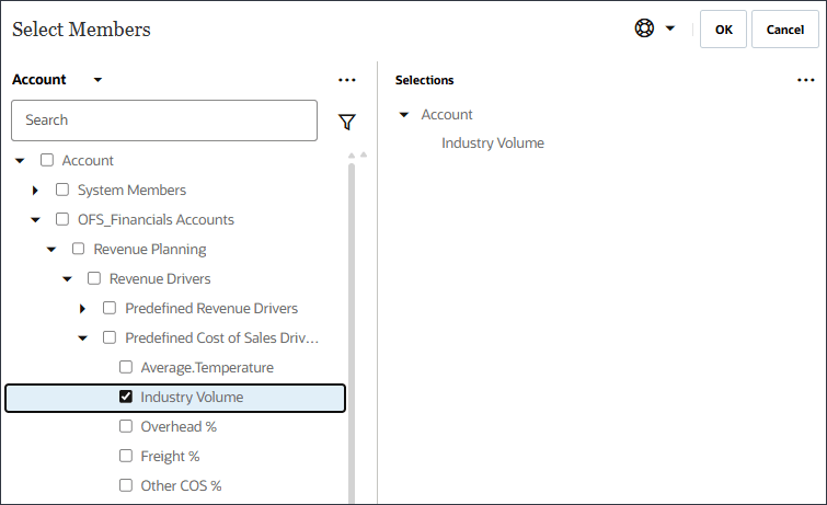
Caution:
Ensure you select the correct Industry Volume account which is under Predefined Cost of Sales Drivers in the hierarchy. - Click Add Driver.
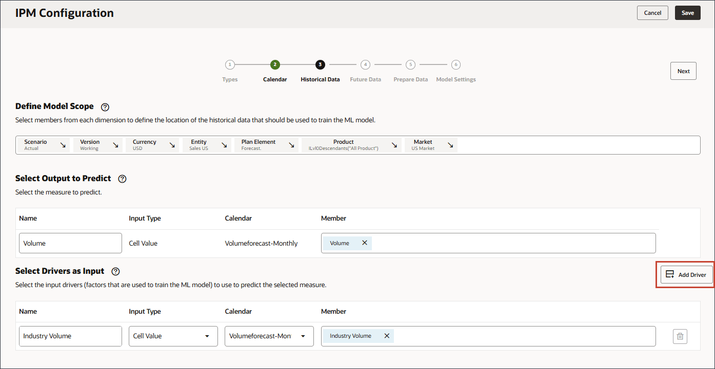
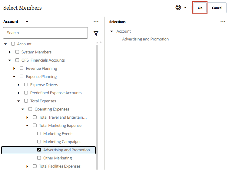
- In Name, enter Advertising and Promotions, and for Advertising and Promotions, in Member, click Industry Volume.
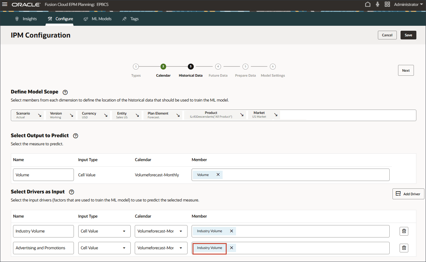
- Select Advertising and Promotion, and click OK.
Tip:
Be sure to select the member with the member name "OFS_Advertising and Promotion". The alias is Advertising and Promotion. - Click Add Driver.
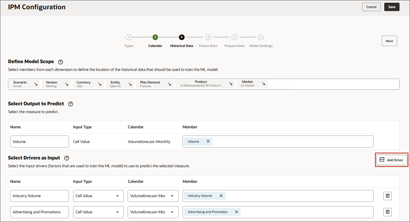
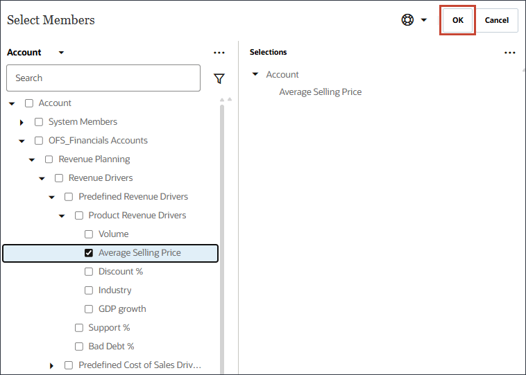
- In Name, enter Average Selling Price, and for Average Selling Price, in Member, click Industry Volume.

- Select Average Selling Price, and click OK.
Tip:
Be sure to select the member with the member name "OFS_Ave Selling Price". The alias is Average Selling Price. - Click Add Driver.

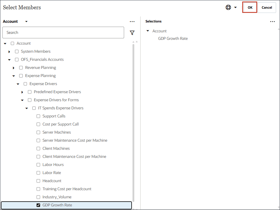
- In Name, enter Economic Indicator, and for Economic Indicator, in Member, click Industry Volume.

- Select GDP Growth Rate, and click OK.
Caution:
Ensure you select the correct account. The member name for this account is Economic Indicator while the alias is GDP Growth Rate.The member Economic Indicator is mapped to GDP Growth Rate.
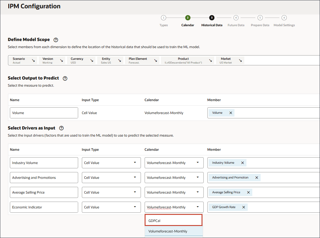
- For Economic Indicator, for Calendar, click Volumeforecast-Monthly, and select GDPCal.
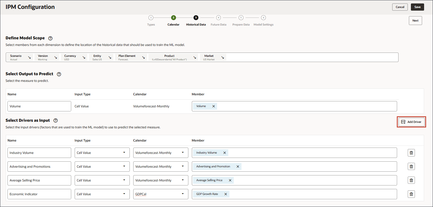
- Click Add Driver.
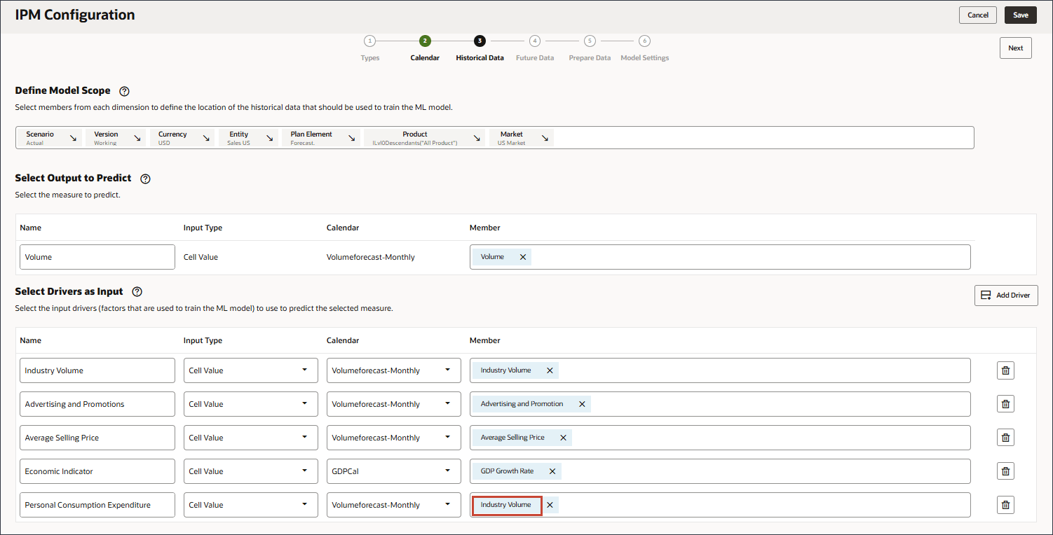
- In Name, enter Personal Consumption Expenditure, and for Personal Consumption Expenditure, in Member, click Industry Volume.
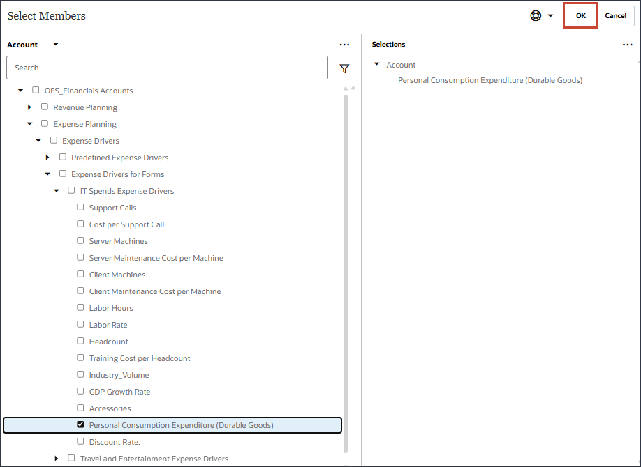
- Select Personal Consumption Expenditure (Durable Goods), and click OK.
Tip:
Be sure to select the member with the member name "Personal Consumption Expenditure (Durable Goods)". The alias for this member is also "Personal Consumption Expenditure (Durable Goods)". - Click Add Driver.
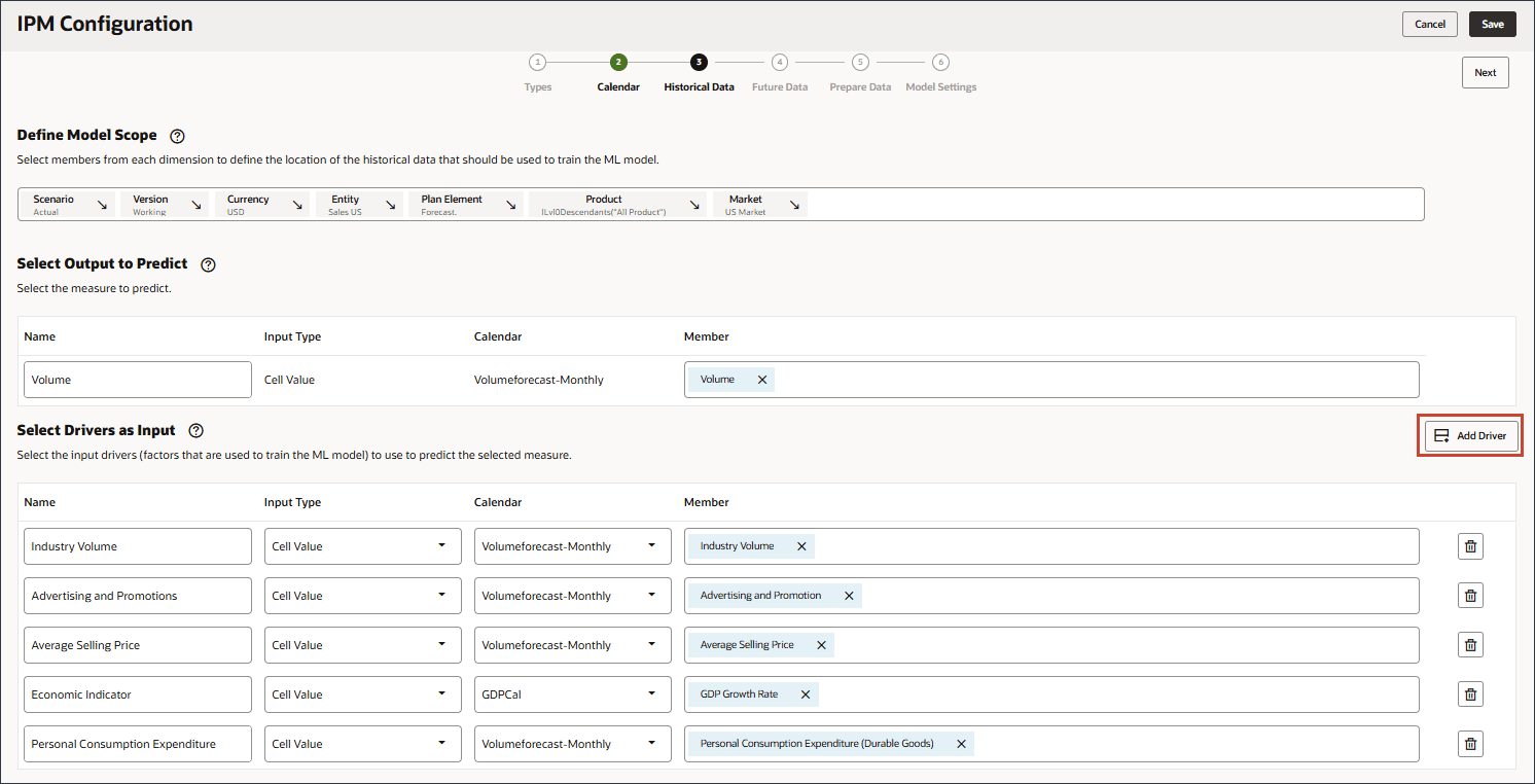
- In Name, enter Discount Rate, and for Discount Rate, in Member, click Industry Volume.
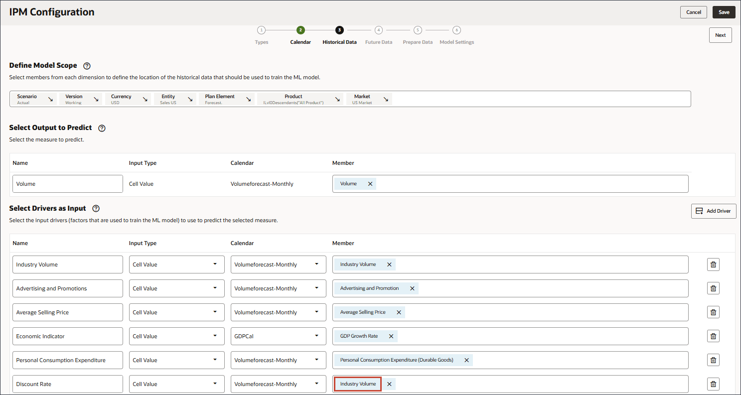
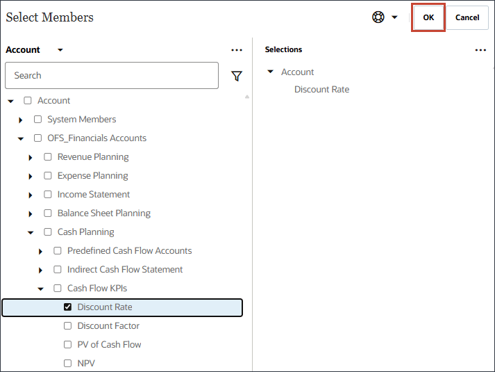
- Select Discount Rate, and click OK.
Tip:
Be sure to select the member with the member name "OFS_Discount Rate". The alias for this member is "Discount Rate" with no period in the name. - Click Add Driver.
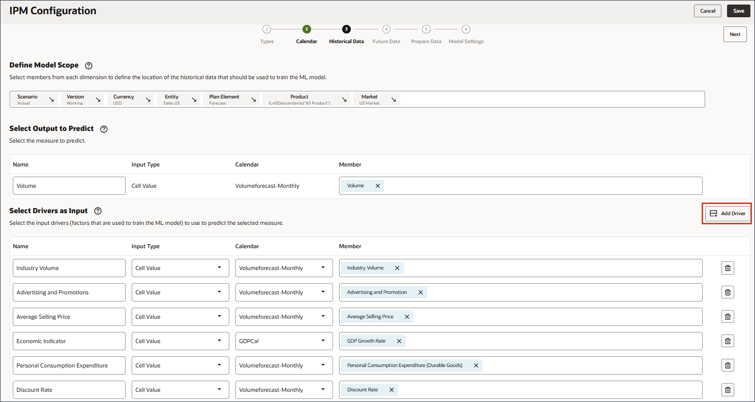
- In Name, enter Accessories and for Input Type, click Cell Value, and select Smart List.

- For Accessories, in Member, click Industry Volume.

- Select Accessories., and click OK.
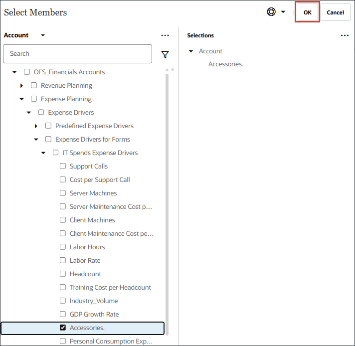
Tip:
Be sure to select the member with the member name "Accessories.". Both the member name and alias are the same, and for both the name includes a period. - Scroll up and click Next.
Selecting the Slice Definition for Future Data
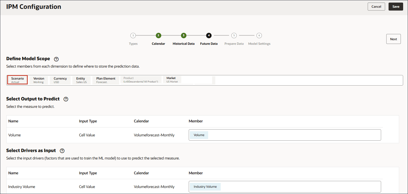
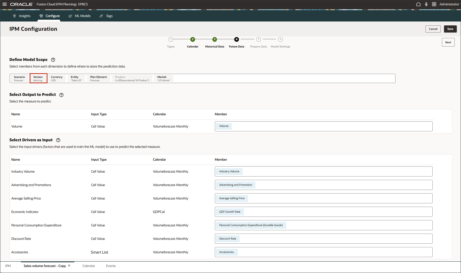
In this section, you select the slice definitions where you want to store the output from predictions. By default, the configuration you set up for historical data is carried forward to the Future Data page. You can modify specific members to define where future data exists as well as where the predictions are stored.
- In the POV, click Scenario.
- Select Forecast, and click OK.
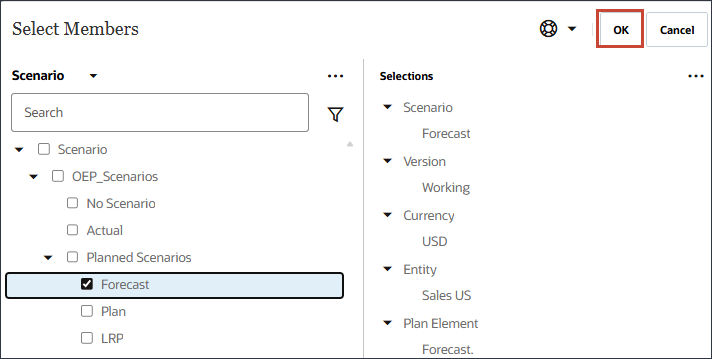
No other changes are needed. Input and output drivers are the same
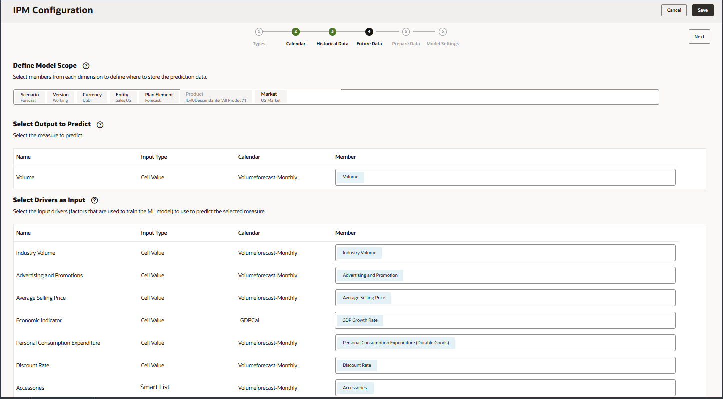
Predicted output can go to the Forecast scenario or any scenario where you want to store predictions.
- Click Next.

Defining Methods for Processing Data Quality Issues
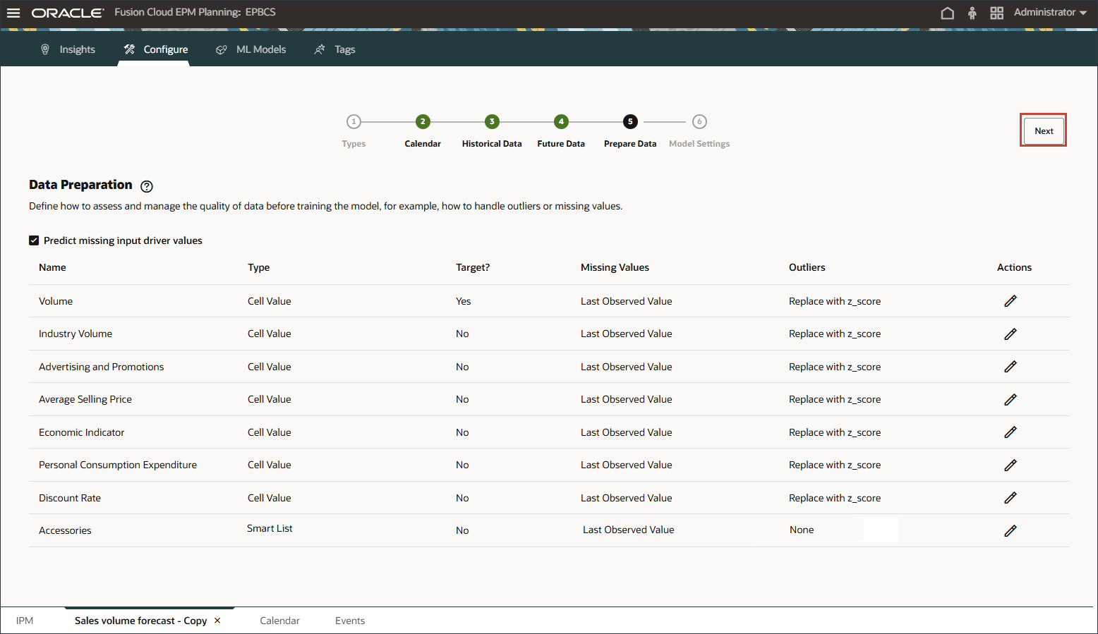
In the data preparation stage, you can select how to handle missing input driver values. Earlier, you reviewed the input drivers, and noticed that there were no future driver data values for the product ‘eReader’.
Data preparation includes columns for the driver name, type, target, missing values, outliers, and Actions.
Define how to assess and manage the quality of data before training the model, for example, how to handle outliers or missing values.
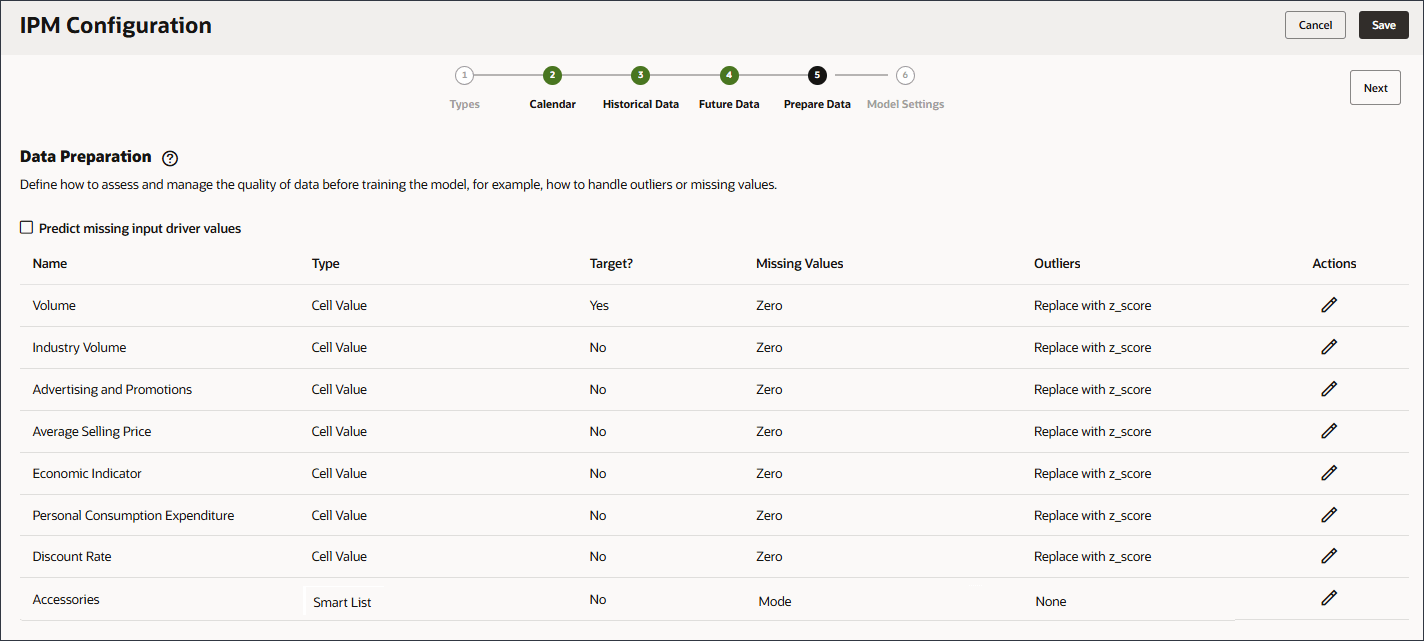
It is quite common for the historical data used for predicting values to be missing values. The data might be missing values for a few reasons, including measurement failures, formatting problems, human errors, or a lack of information to record. There are different provided filling options to handle missing values in your target predictions and related datasets. Filling is the process of adding standardized values to missing entries in the dataset.
You can choose from the following options to replace missing values:
- None: No action to be taken (send the data as-is).
- Zero: Replace missing values for any column with zero.
- Replace with Mean (Numeric Data): Replace with Mean across the historical series.
- Replace with Median (Numeric Data): Replace with Median point of the historical series.
- Replace with Mode (Numeric and Categorical Data): Replace with the most common value in historical data.
- Replace with Next Observed Value: Replace missing values with the value observed/seen in the next period.
- Replace with Last Observed Value: Replace missing values with the value that was observed in the previous period.
For Outliers, you define whether the system should replace it with zero, mean, z-score or none.
The following options can be seleted to replace an outlier:
- None: No outliers treatment to be done.
- Replace with Zero: Replace with 0.
- Replace with Mean: Replace with mean of K nearest values.
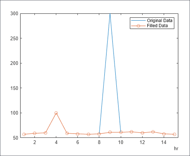
- Replace with Z score: For any numerical column, any value falling out of mean +/- 3*Standard Deviation (std dev) is treated as an outlier. A value less than 'mean - 3*std dev' will be replaced with 'mean -3*std dev'. Similarly, a value greater than 'mean + 3*std dev' is replaced by 'mean + 3*std dev'.
In the graph below is an example of an outlier that is identified and replaced with a normalized value.
- Enable Predict missing input driver values.
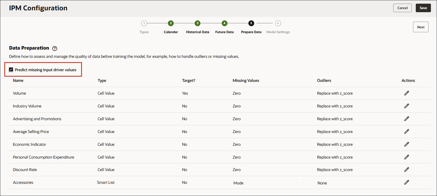
By enabling Predict missing input driver values, the values are predicted using statistical forecasting, namely univariate predictions if data does not exist for those measures.
- For Missing Values, notice the list of options.
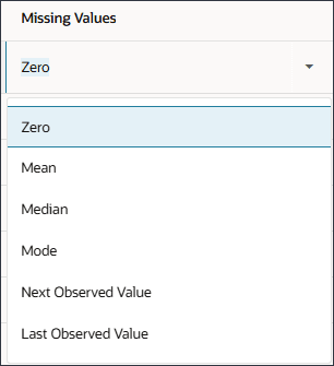
If you want to modify the selection for Missing Values, for the driver row, in the Actions column, click
 (Actions).
 - For each of the driver rows, in Actions, click
 (Actions), and in the options list, select Last Observed Value.
 - For Outliers, notice the list of options.
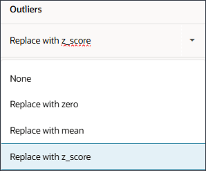
If you want to modify the selection for Outliers, for the driver row, in the Actions column, click
 (Actions).
 - Click Next.
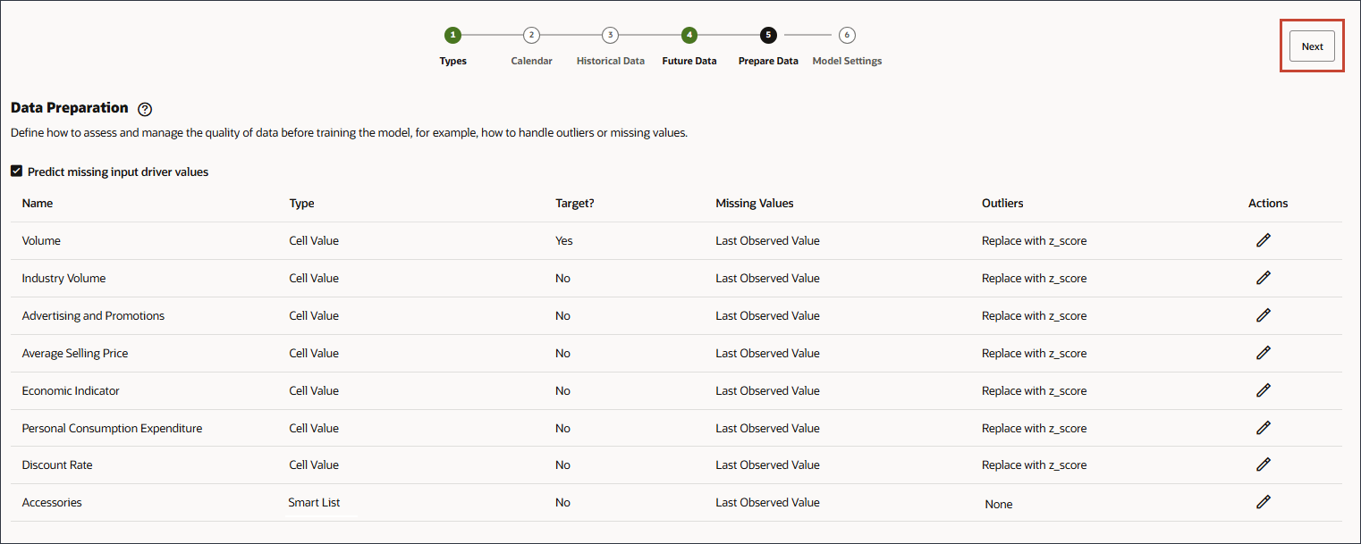
Tip:
After changing each row's Missing Values option, you can clickMissing Values for all the drivers are set to Last Observed Value.
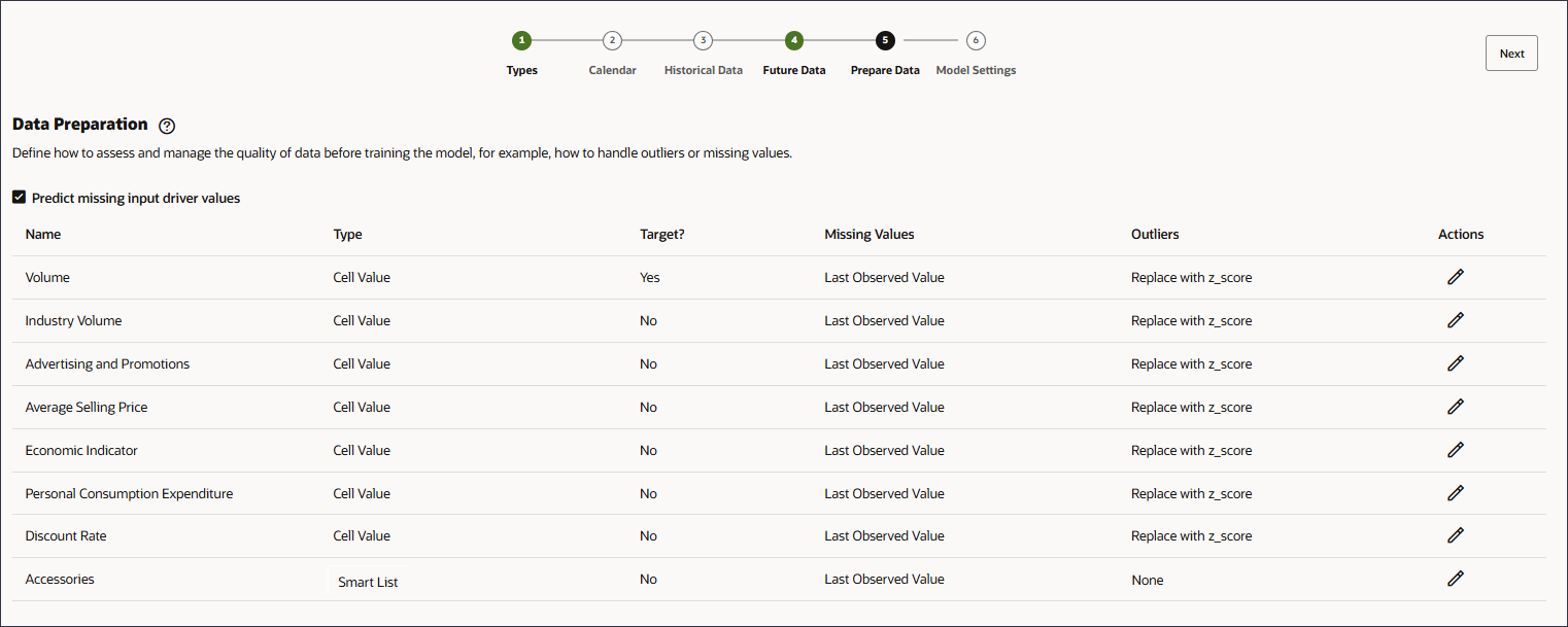
Selecting Algorithms for Model Settings
In this section, you select the algorithms for model settings.
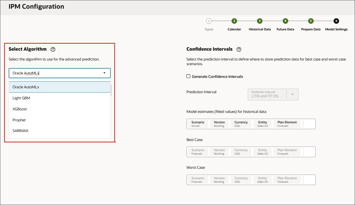
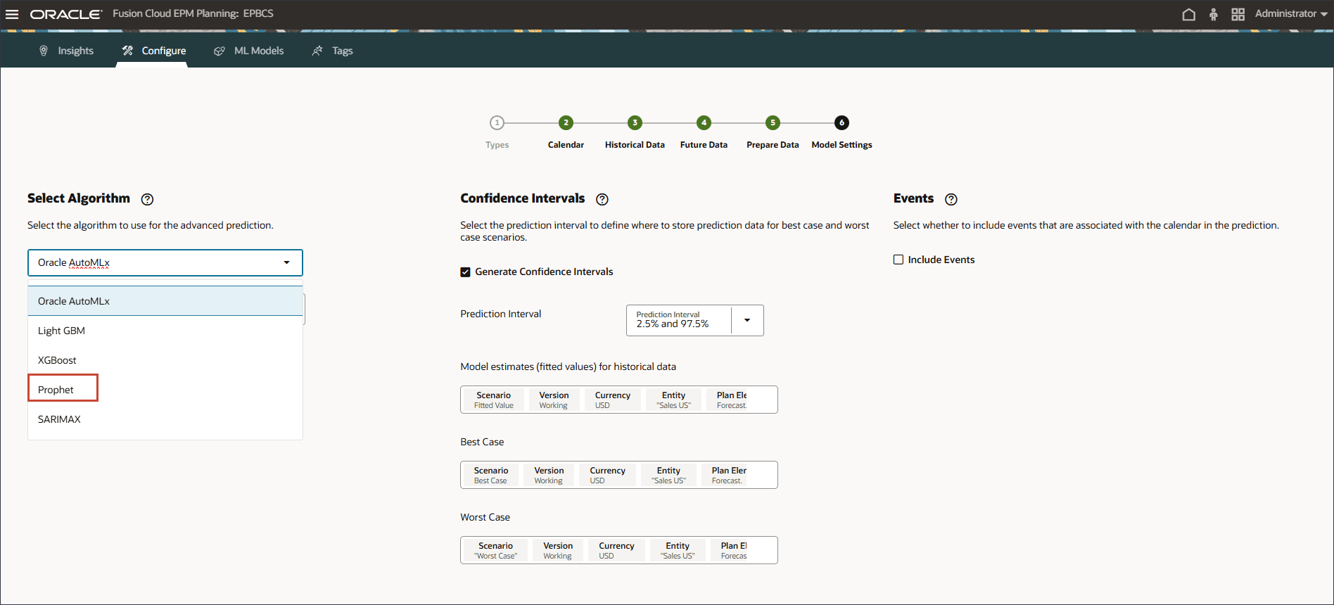
You can select Oracle AutoML or specific algorithms such as Light GBM, XGBoost, Prophet, or SARIMAX.
Oracle AutoMLx is a proprietary framework that does the following:
- Runs various statistical models and machine learning algorithms on your data
- Tunes and validates the models
- Finds the best model for your data
- Fits your data to the best model

You can select one of various algorithms such as Oracle AutoMLX, Light GBM, XGBoost, Prophet, and SARIMAX. These are best practice Advanced Prediction algorithms available globally for model training. The AutoMLX Algorithm has multiple algorithms as per details below.
The AutoMLX python package automatically creates, optimizes and explains machine learning pipelines and models. The AutoML pipeline provides a tuned ML pipeline that finds the best model for a given training dataset and a prediction task at hand. AutoML has a simple pipeline-level Python API that quickly jump-starts the data science process with an accurately tuned model. AutoML has support for any of the following tasks:
- AutoClassifier: Supervised classification or regression prediction with a tabular dataset where the target can be a simple binary or a multi-class value or a real valued column in a table, respectively.
- AutoRegressor: Supervised classification for Image and Text datasets.
- AutoAnomalyDetector: Unsupervised anomaly detection, where the target or the labels are not provided.
- AutoForecaster: Univariate and multivariate timeseries forecasting task.
The AutoML pipeline consists of five major stages of the ML pipeline: pre-processing, algorithm selection, adaptive sampling, feature selection, and model tuning. These pieces are readily combined into a simple AutoML pipeline which automatically optimizes the whole pipeline with limited user input/interaction.
EPM’s Advanced Prediction leverages AutoML’s AutoForecaster package under the hood.
List of algorithms in AutoForecaster:
- NaiveForecaster
- ThetaForecaster
- ExpSmoothForecaster
- ETSForecaster
- STLwESForecaster
- STLwARIMAForecaster
- SARIMAXForecaster – Multivariate
- ExtraTreesForecaster - Multivariate
- XGBForecaster (XG Boost) – Multivariate
- LGBMForecaster (Light Gradient Boosting Machine) – Multivariate
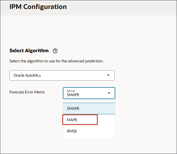
Forecast error metric selection uses your choice of error measure:
- RMSE: Root Mean Squared Error
- MAPE: Mean Absolute Percentage Error
- MAD: Mean Absolute Deviation
The forecast error metric chooses the model with the least error as the best model.
For the best model:
- Generates fitted series corresponding to the input series.
- Generates forecast for the horizon.
- In Select Algorithm, click the drop-down list to view the selections, and then select Oracle AutoMLx.
- For Forecast Error Metric, for Metric, select MAPE.
Selecting Confidence Intervals for Model Settings
In this section, you select confidence intervals, and metrics for which to optimize.
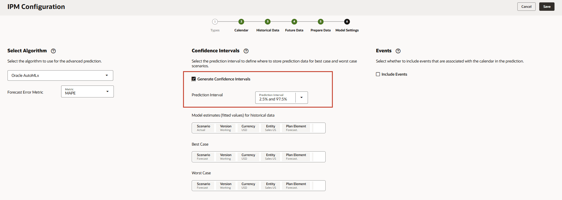
Based on the confidence intervals settings, the system generates multiple scenarios of Advanced Predictions and stores the results according to the provided scenario in this model settings setup.
- The confidence intervals in prediction can provide an upper and lower bound for predicted output values.
- For example, using the confidence intervals of 10% (P10) and 90% (P90) provides a range of values known as an 80% confidence interval. The observed value is expected to be lower than the P10 value 10% of the time, and the P90 value is expected to be higher than the observed value 90% of the time.
- By generating forecasts at P10 and P90, you can expect the true value to fall between those bounds 80% of the time. This range of values is depicted by the shaded region between P10 and P90 in the figure shown.

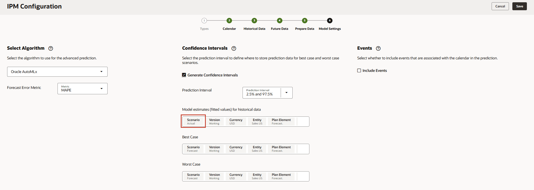
- On the Model Settings page, in Confidence Intervals, select Generate Confidence Intervals.
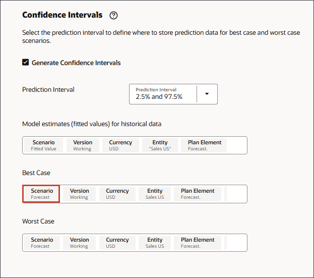
- For Prediction Interval, keep the default settings for the Best Case, Worst Case, and Fitted value predictions.
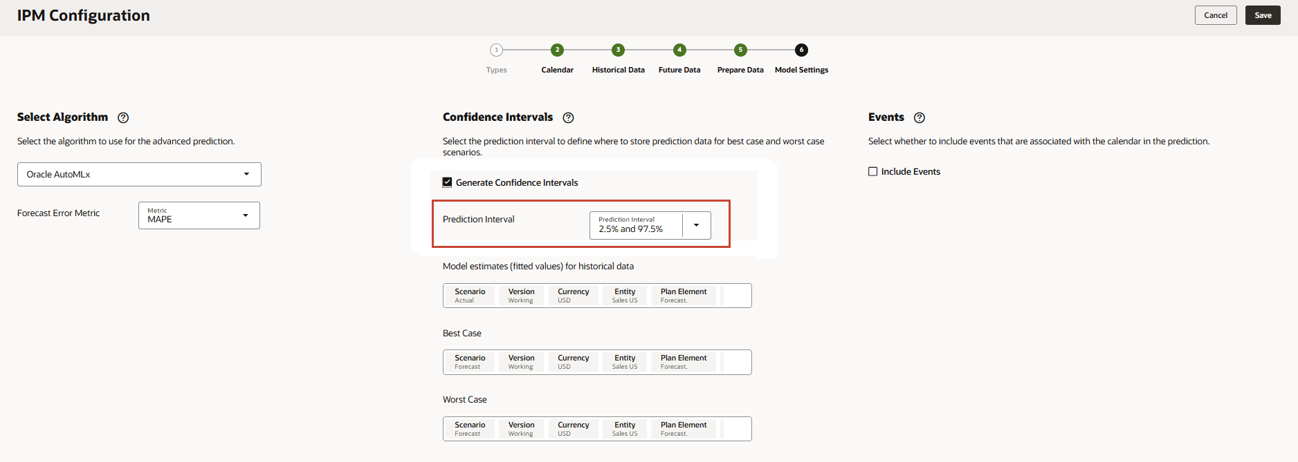
- In Model estimates (fitted values) for historical data, click Scenario.
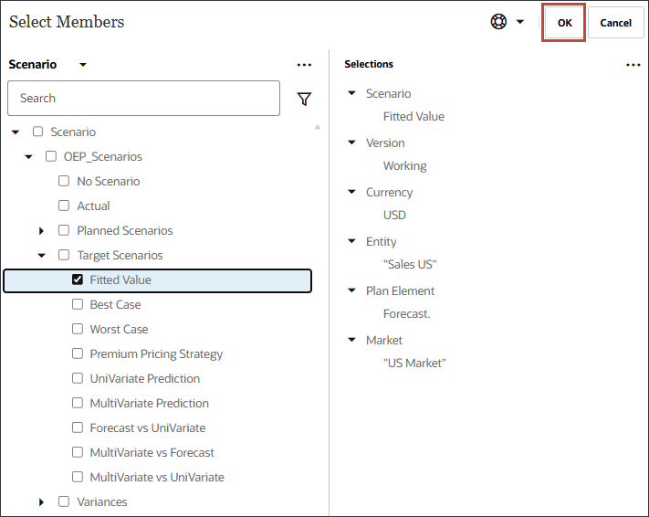
- For Scenario, select Fitted Value, and click OK.
- In Best Case, click Scenario.
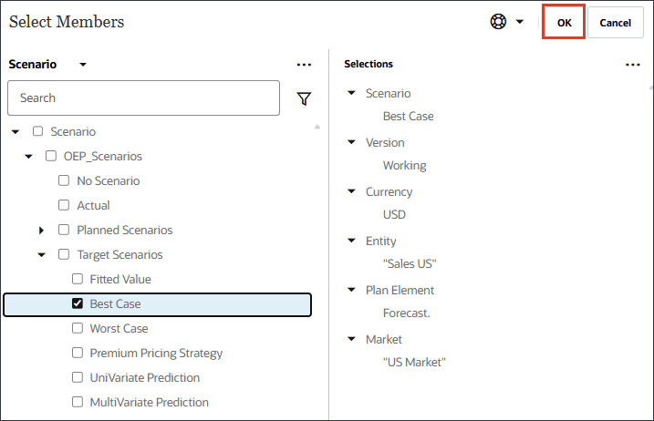
- For Scenario, select Best Case, and click OK.
- In Worst Case, click Scenario.
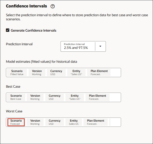
- For Scenario, select Worst Case, and click OK.
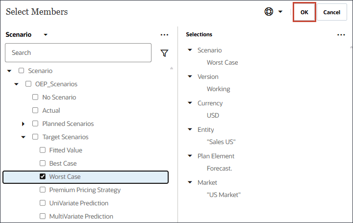
Selecting Events
In this section, you select whether to include events in the prediction.
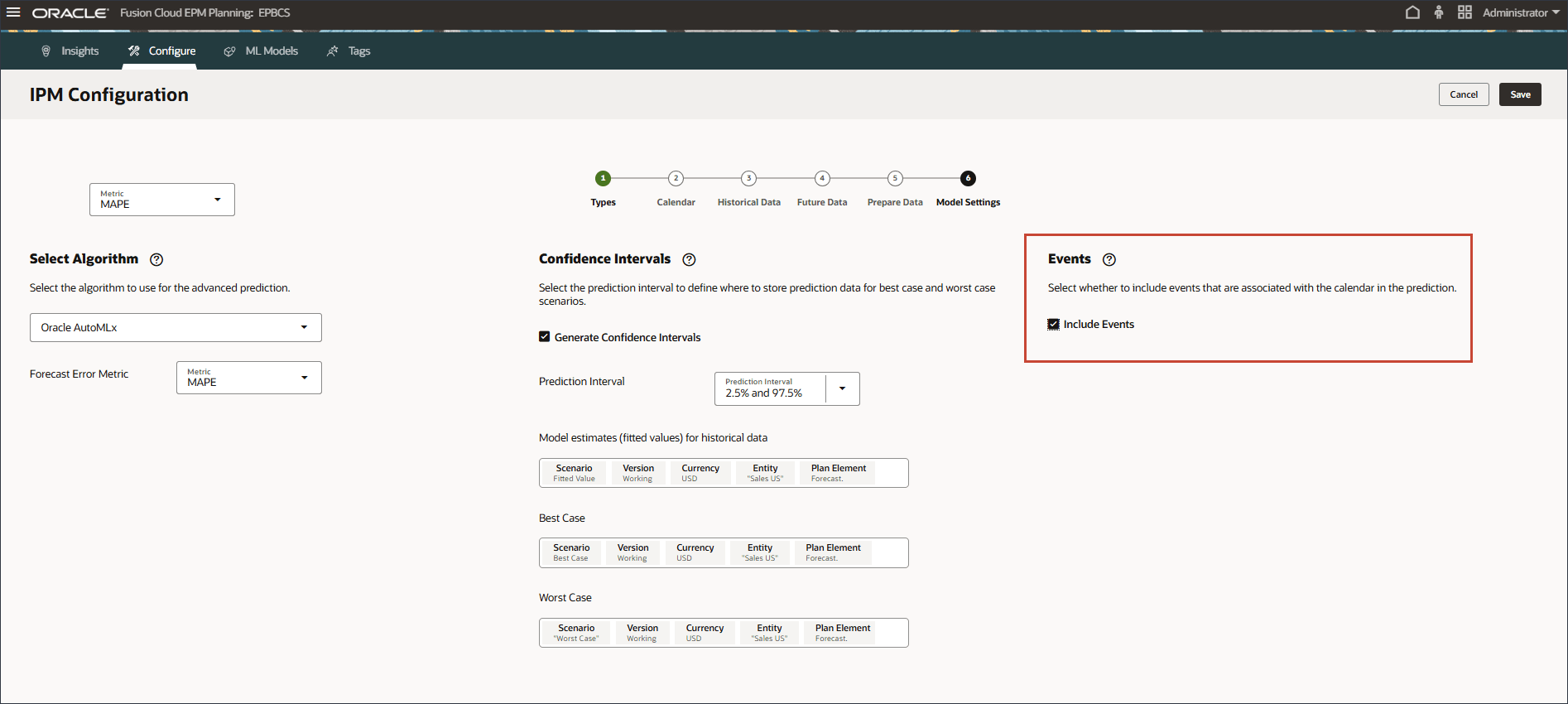
You can include events in your predictions. Events can be used for advanced tuning and for improving accuracy if you want certain events that occur and impact the past data to be considered for predictions. These events can include:
- Recurring events in same periods such as Christmas
- Recurring events in varying periods such as Ramadan
- One-off events such as hurricanes
- Skip events such as the pandemic
- On the right, under Events, select Include Events.
- Click Save.
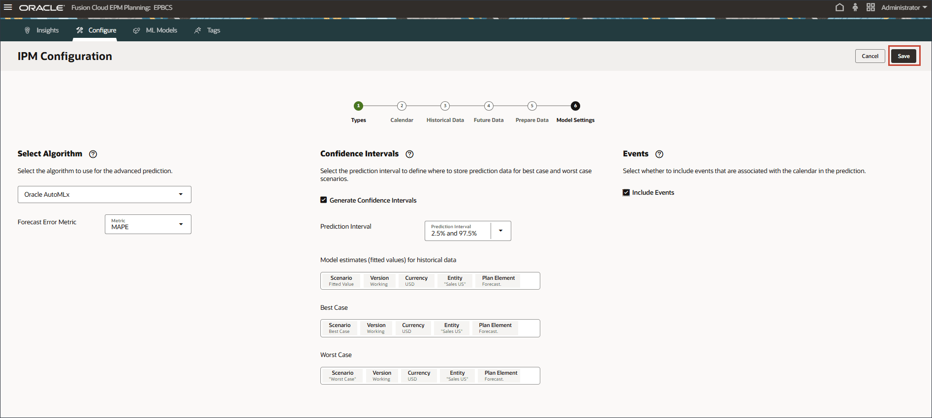
An Information message is displayed.

- Click Cancel.
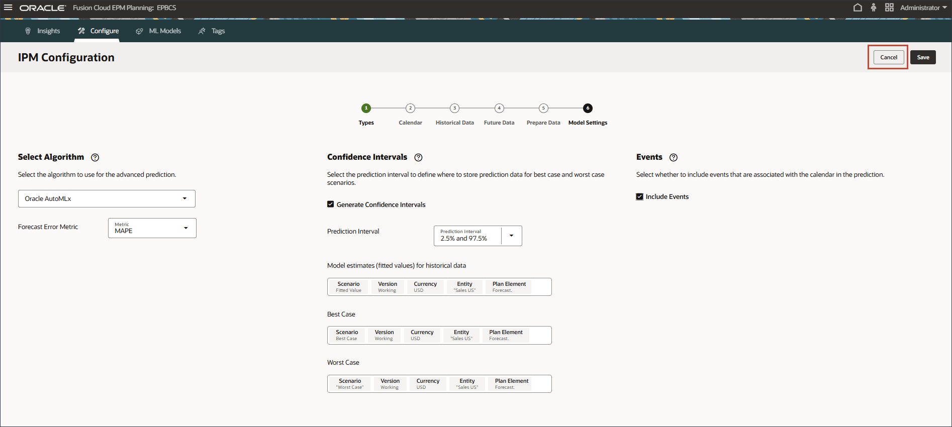
The new Advanced predictions job is displayed.

Adding Events
In this section, you add a new marketing campaign event for period May-22, Jul-23 and Sep-24. While May-22 and Jul-23 are actual periods, Sep-24 is a future prediction period where a marketing campaign is planned to happen. The event is essentially indicating that the same event that happened in May and July in previous years, is also planned to occur in Sept in the future year.
- Click the Events tab.

- Click Add Event.
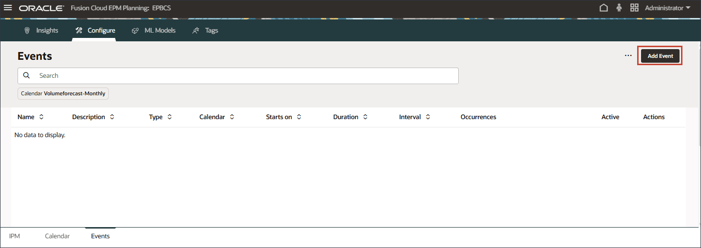
- For the new event, enter or select the following information:
Column Value Name Marketing Campaigns Description Marketing Campaigns Type Repeat Calendar Volumeforecast-Monthly Duration 1 The Marketing Campaigns event is of type Repeat, and is based on the Volumeforecast-Monthly calendar.

- For Occurrences, click
 (Event Occurrences).

- Select Custom, and click Select periods.
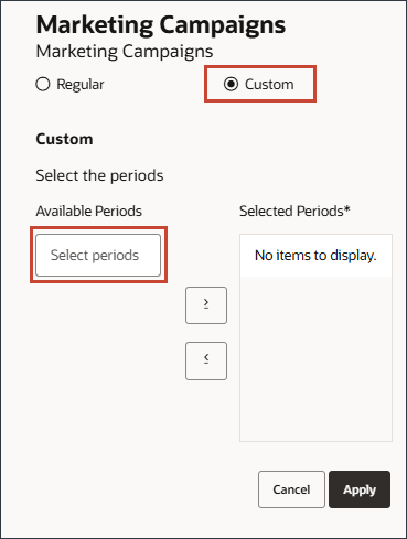
- For periods, select May FY22, and move it to selected periods.
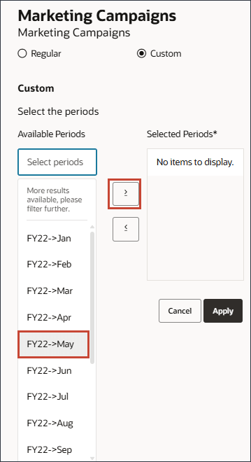
- On the left, click in the period area, and type FY23.
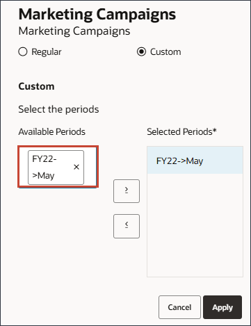
A search box is displayed.
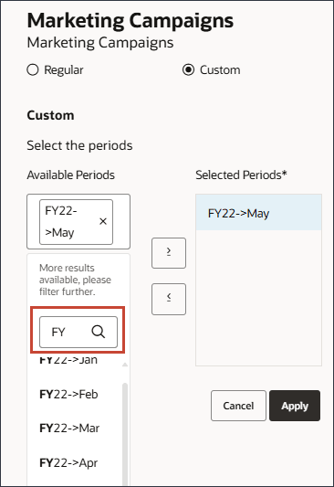
- Select Jul FY23.
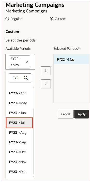
- Click in the Available Periods area, and type FY24, and select Sept FY24.
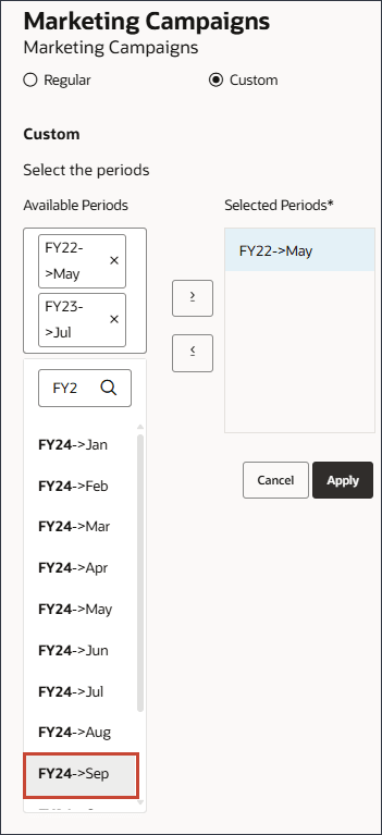
- Move all periods to Selected Periods.
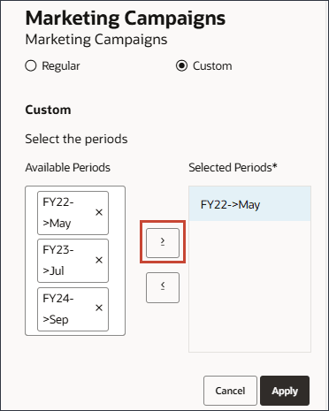
- Click Apply.
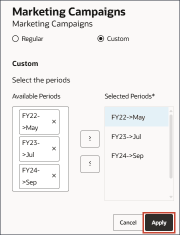
- On the right in the row for the new event, click
 (Save).

- Click
 (Home) to return to the Home page.
Reviewing Advertising and Promotion Cost and Sales Volume
In this section, you review the actual data for Advertising and Promotion cost and sales volume for the months of May 2022 and July 2023, to understand the correlation between the driver and the output. You also review future September 2024 driver data.
- On the home page, click Advanced Predictions, and then Volume Prediction.

- Select the Input Drivers tab.
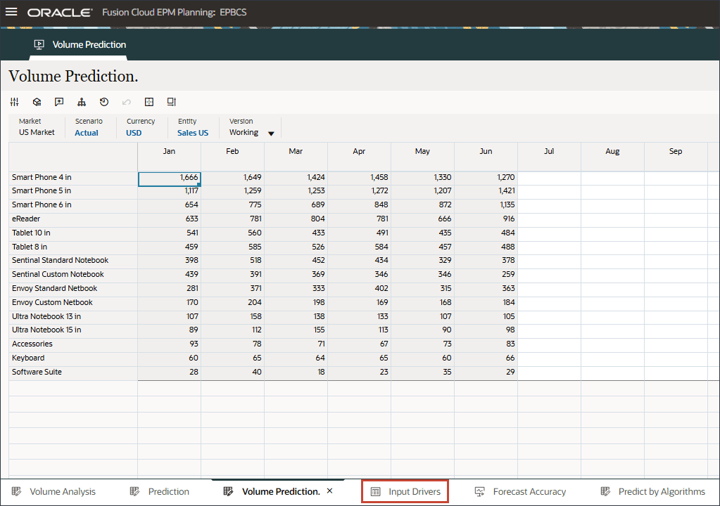
- In the POV, click Account, and select Advertising and Promotion.
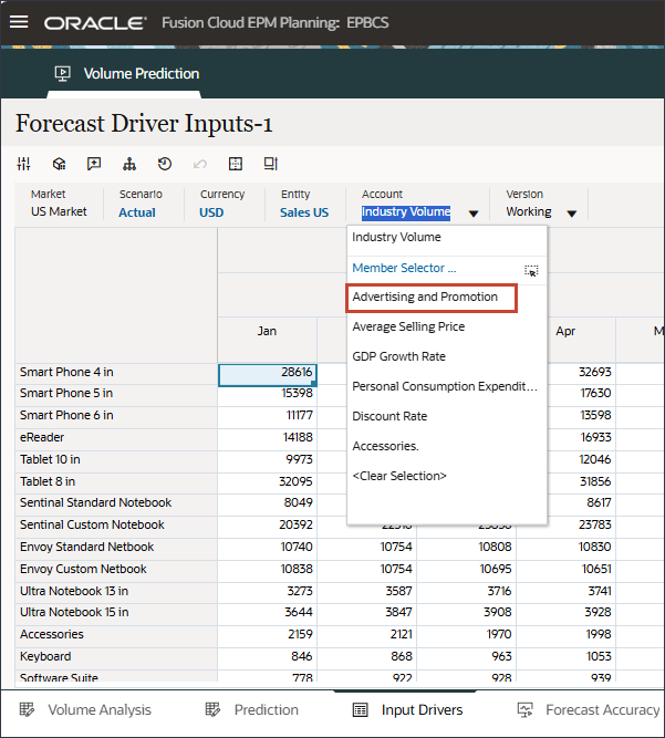
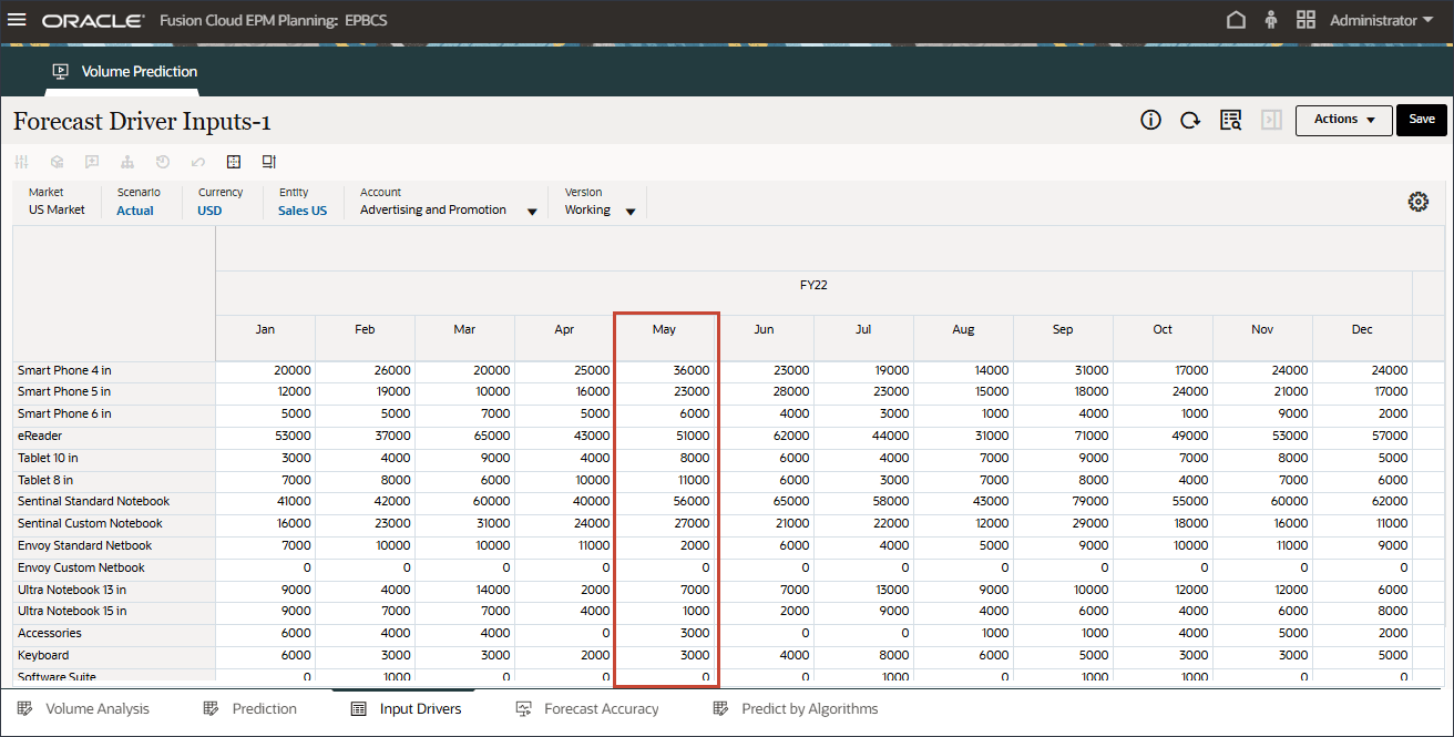
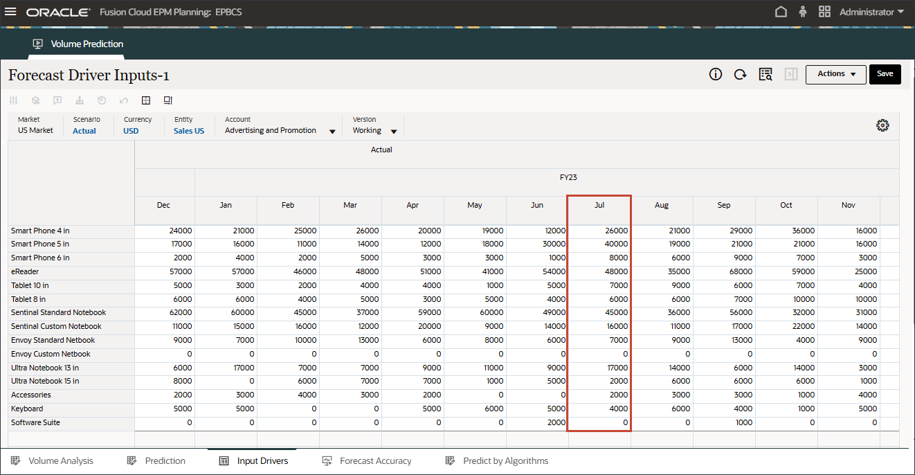
- For May 22 and July 23, the data is bumped up for those months.
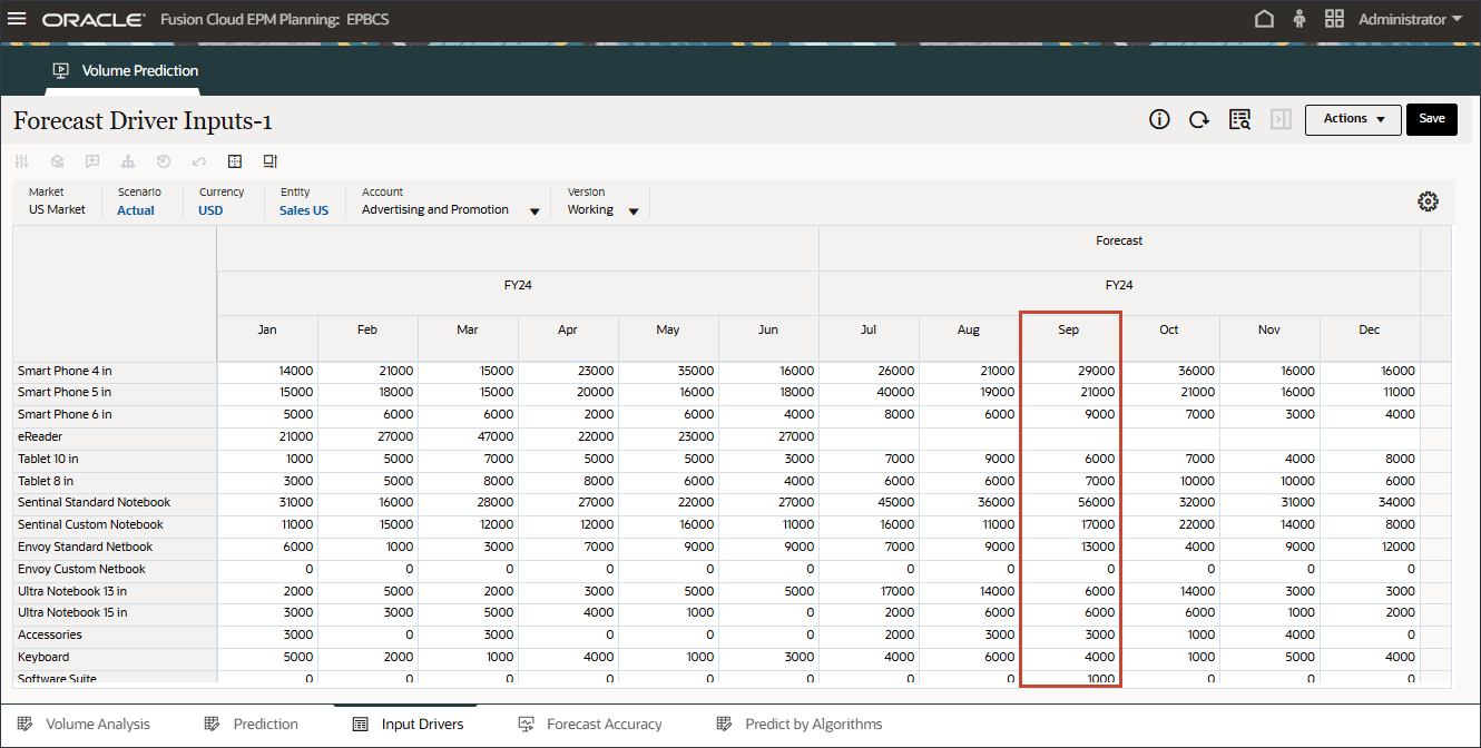
For future September 2024 data, the system should automatically bump up the prediction results since Events were enabled in the configuration job.
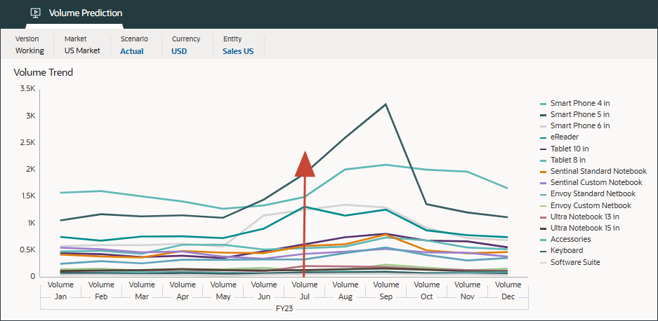
- On the bottom of the page, click the Volume Analysis tab.
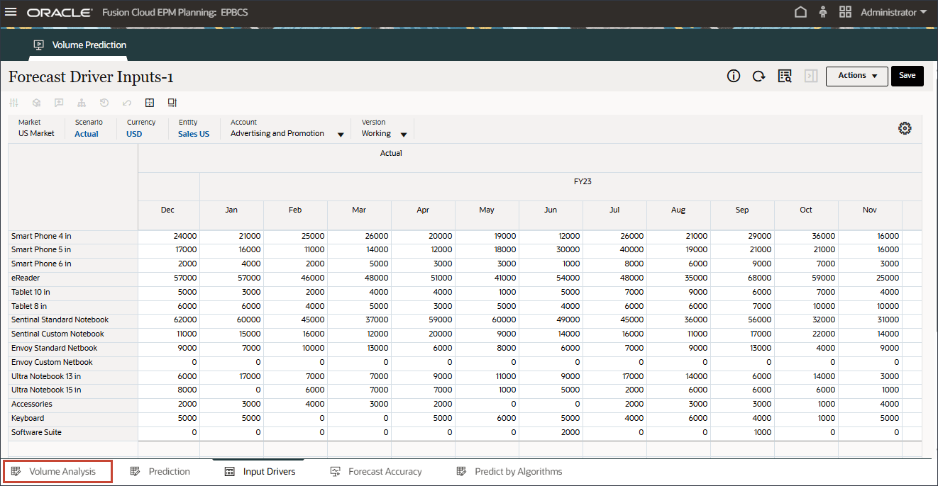
The Volume analysis chart shows the July 2023 volume data is bumped up due to the marketing campaign event.
- Click
 (Home) to return to the Home page.
Running the Advanced Prediction Job
In this section, you run the Advanced Prediction job to generate predictions.
- On the home page, click IPM, and select Configure.

- On the bottom, select the IPM tab.

- For Sales volume forecast, on the right, click
 (Actions), and select Run.

On the IPM page, you can run the advanced prediction job, monitor the status of the job, review the error log, and make changes to the configuration as required.
- After you run the job, an Information message is displayed letting you know that the job has been started successfully.

In the Last Run column, where there is a date and time, you can view the current status. After submitting the job, "Processing" is the displayed status.

- On the IPM page, click Refresh to update the job status.

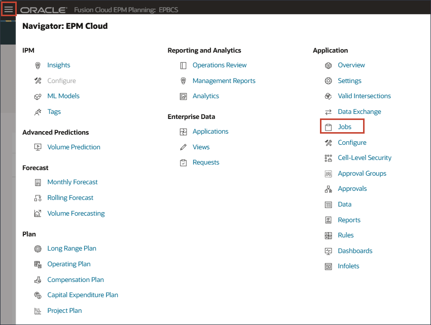
- Click
 (Navigator) and under Application, click Jobs.
- On the Jobs page, click Sales volume forecast.

Multiple jobs were triggered internally to generate the predictions.
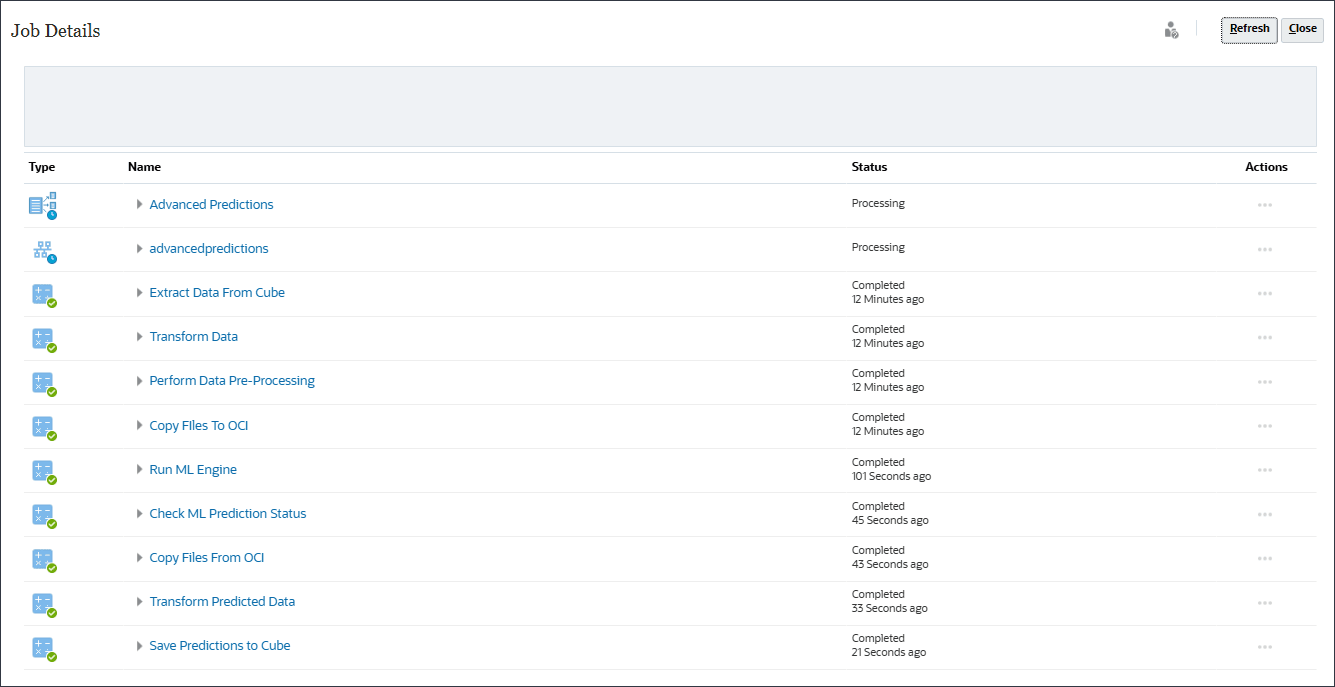
With just one click, the system tests multiple algorithms, including exponential smoothing, ARIMA, and regression models, then surfaces the most statistically accurate forecast. This empowers planners to produce data-driven forecasts in seconds, replacing hours of manual analysis.
- Wait until all the Advanced Prediction jobs are completed successfully, and click Close.

The main job completed successfully.

- Click
 (Navigator) and under IPM, click Configure.
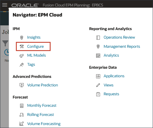
Sales volume forecast completed successfully.

- After the job completes successfully, you can download the report and review the prediction results. For Sales volume forecast, on the right, click
 (Actions), and select Download Report.

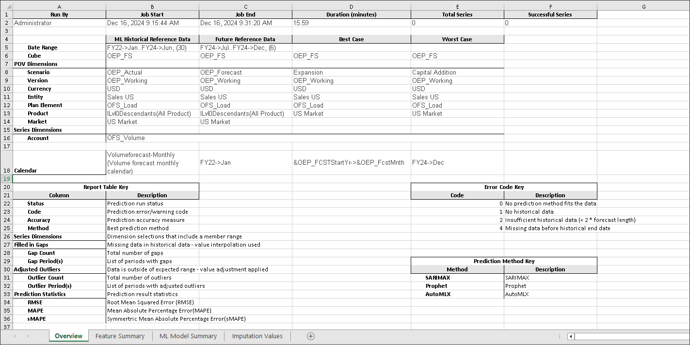
The download report is a zip file which includes a .csv file with all the details related to the Advanced Prediction job. You can review this sample Sales volume forecast report.
Below is a sample from the report.
- Click
 (Home) to return to the Home page.
Note:
The job takes a few moments to complete.Note:
The job takes a few moments to complete.Reviewing Advanced Prediction Results
Reviewing Volume Forecast Prediction Results
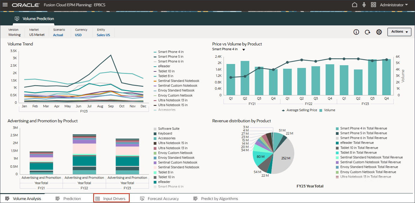
In this section, you review the volume forecast prediction results.You want to ensure that the eReader product category future values were predicted using the Imputation feature "Predict missing input driver values" for all the input driver accounts.
- On the home page, click Advanced Predictions, and select Volume Prediction.

- On the bottom, click the Input Drivers tab.
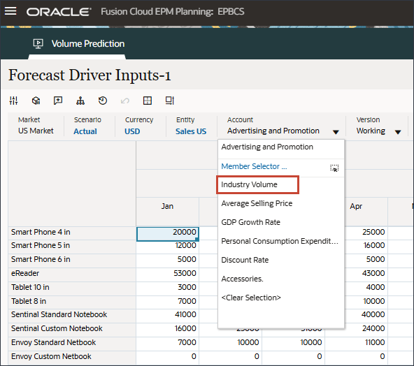
- In the POV, for Account, select Industry Volume.
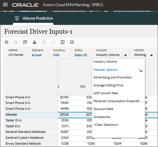
- Scroll to the right.
Industry volume future data (July to Dec, FY24) was predicted using the imputation feature(“Predict missing input driver values”) in the Advanced prediction job.

- In the POV, for Account, select Advertising and Promotion.
Advertising and Promotion data (July to Dec, FY24) was predicted using the imputation feature(“Predict missing input driver values”) in the Advanced prediction job.

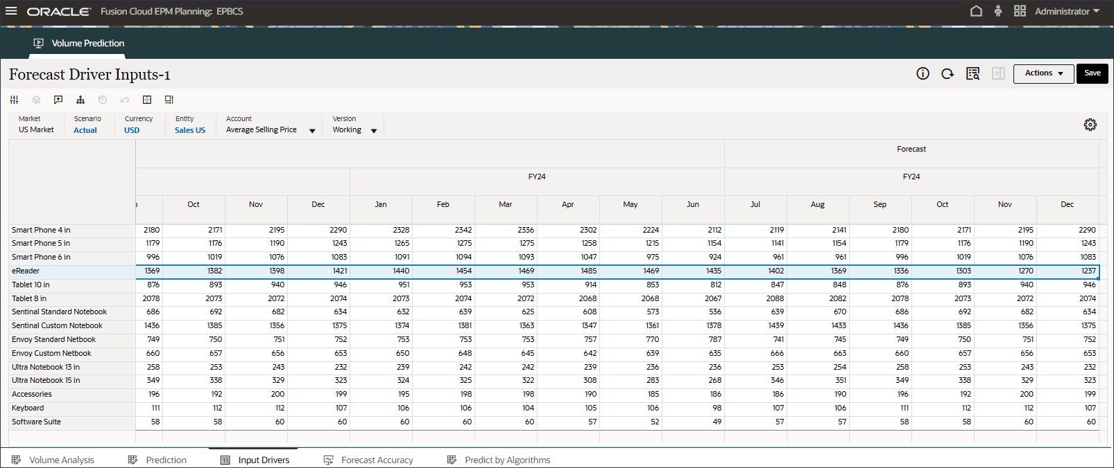
- In the POV, for Account, select Average Selling Price.
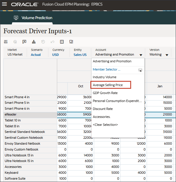
Average Selling Price (July to Dec, FY24) was predicted using the imputation feature(“Predict missing input driver values”) in the Advanced prediction job.
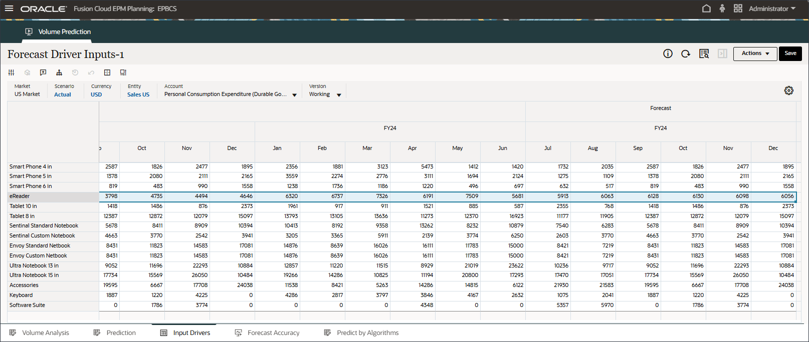
- In the POV, for Account, select Personal Consumption Expenditure (Durable Goods).
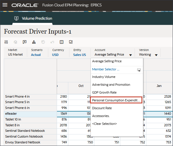
Personal Consumption Expenditure (Durable Goods) (July to Dec, FY24) was predicted using the imputation feature(“Predict missing input driver values”) in the Advanced prediction job.
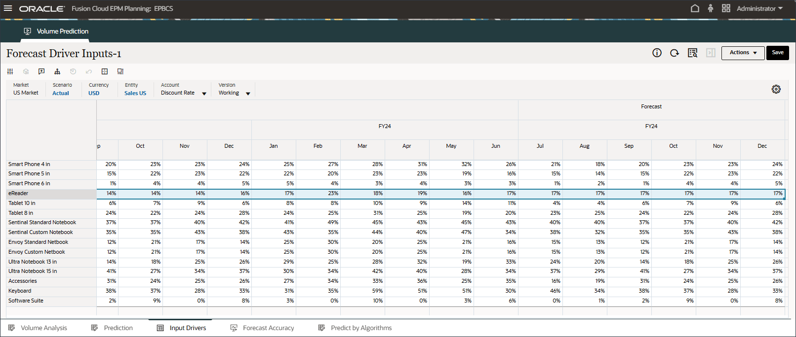
- In the POV, for Account, select Discount Rate.
Discount Rate (July to Dec, FY24) was predicted using the imputation feature(“Predict missing input driver values”) in the Advanced prediction job.
- In the POV, for Account, select Accessories.
Accessories (July to Dec, FY24) was predicted using the imputation feature(“Predict missing input driver values”) in the Advanced prediction job.
Reviewing Prediction Results for Target Variables
In this section, you review the prediction results for the target variable which is Product Sales volumes.
- On the bottom, click the Prediction tab.
The Volume Prediction dashboard is displayed.
- In the middle for the Volume Prediction form, click
 (Actions), and select Open Form.
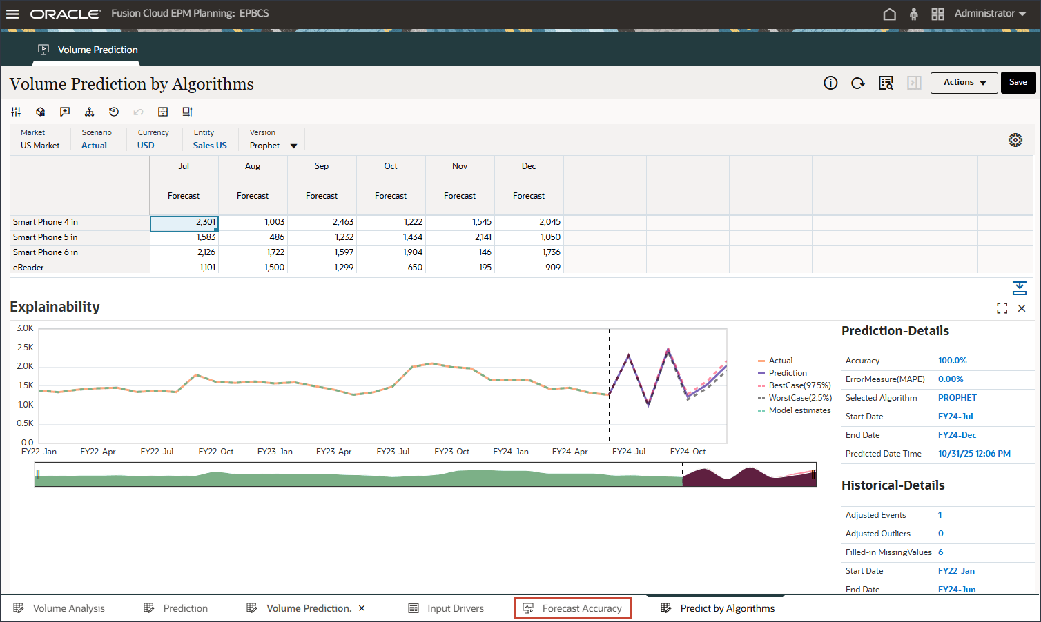
The advanced prediction results are generated from July to December FY24 with the Oracle Auto MLX Algorithm that was configured in the IPM job.
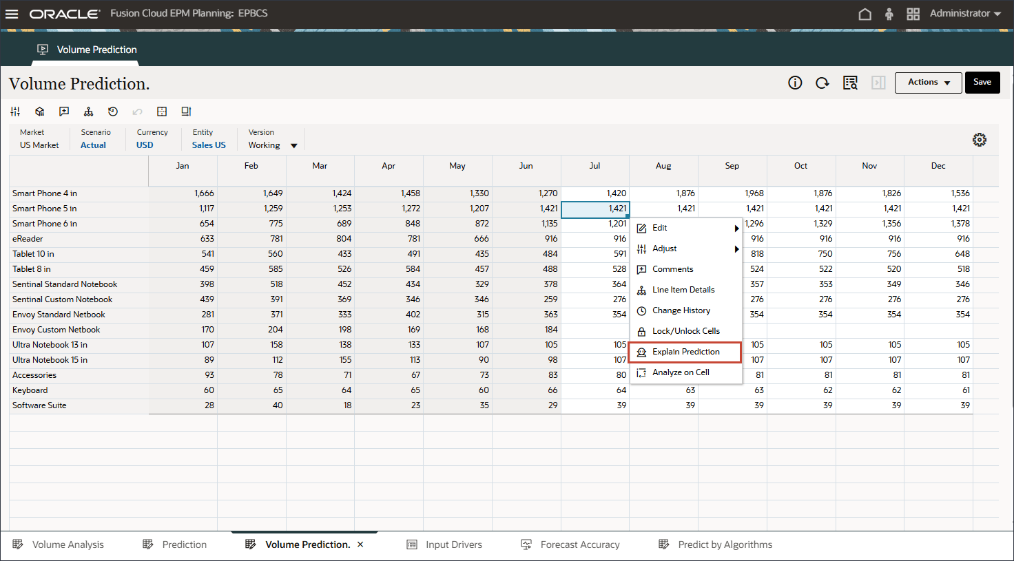
- To review more details and see an explanation on prediction results, right-click in any period such as July for Smart Phone 5 in, and select Explain Predition.
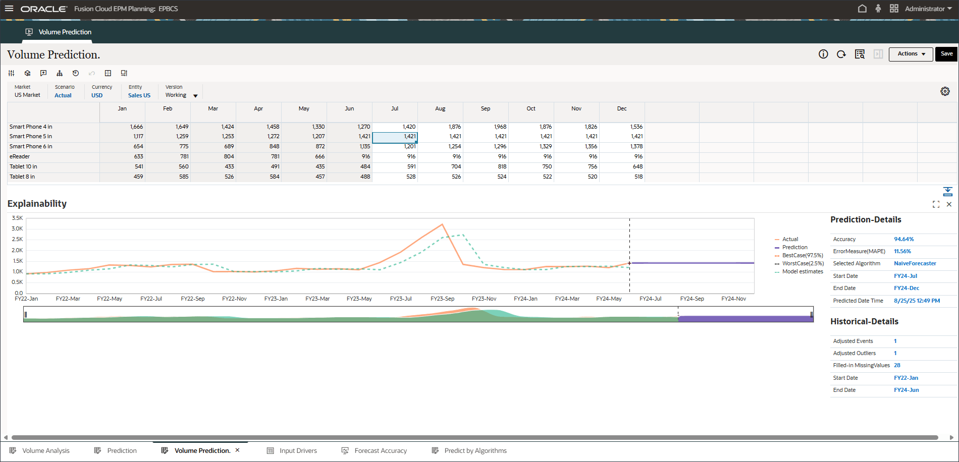
A line chart with historical trend and prediction results considering best case, worst case, most likely scenarios is displayed. Also provided are additional prediction details such as Accuracy%, Error measure(MAPE), Algorithm used in generating prediction results, prediction start and end date.
- Make a different selection such as September for Smart Phone 6 in.
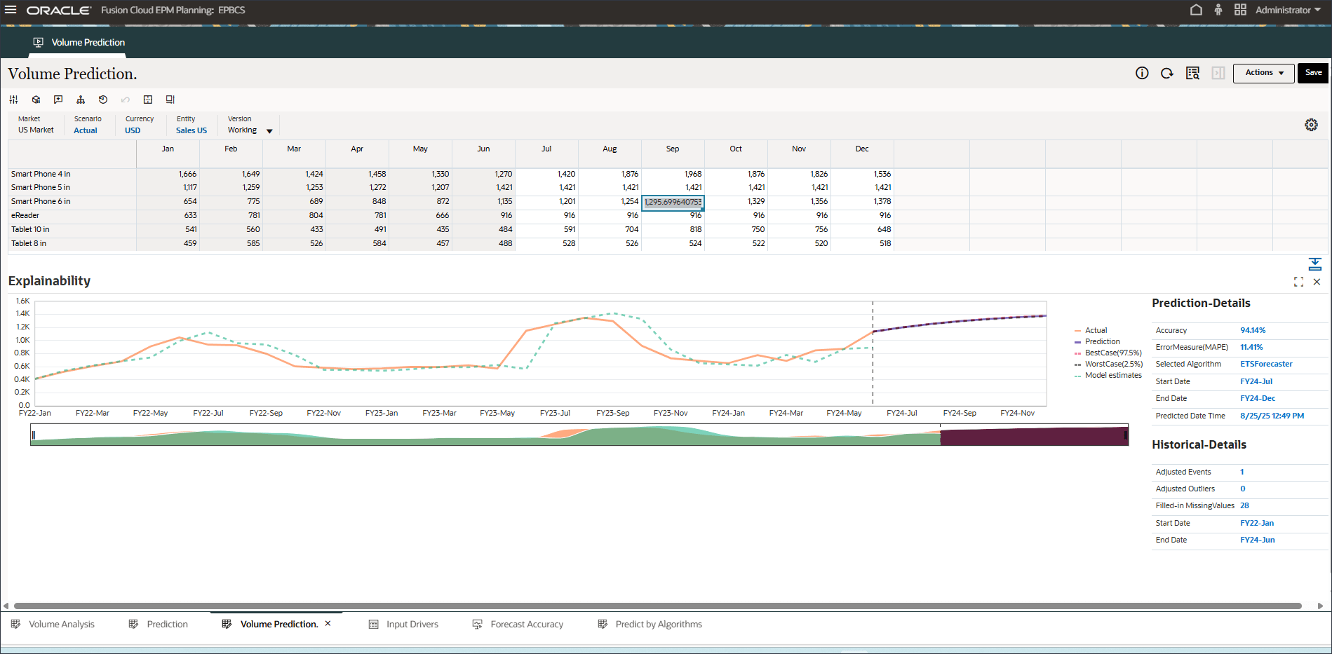
Notice that Oracle Auto MLX uses different algorithms for each product based on accuracy results. Also notice the impact of Events showing up in FY22-May, FY23-Jul and FY24-Sep prediction results.
- If you want to refine the input drivers and rerun the advanced prediction job, you can navigate to the Input Drivers tab and edit the driver values.
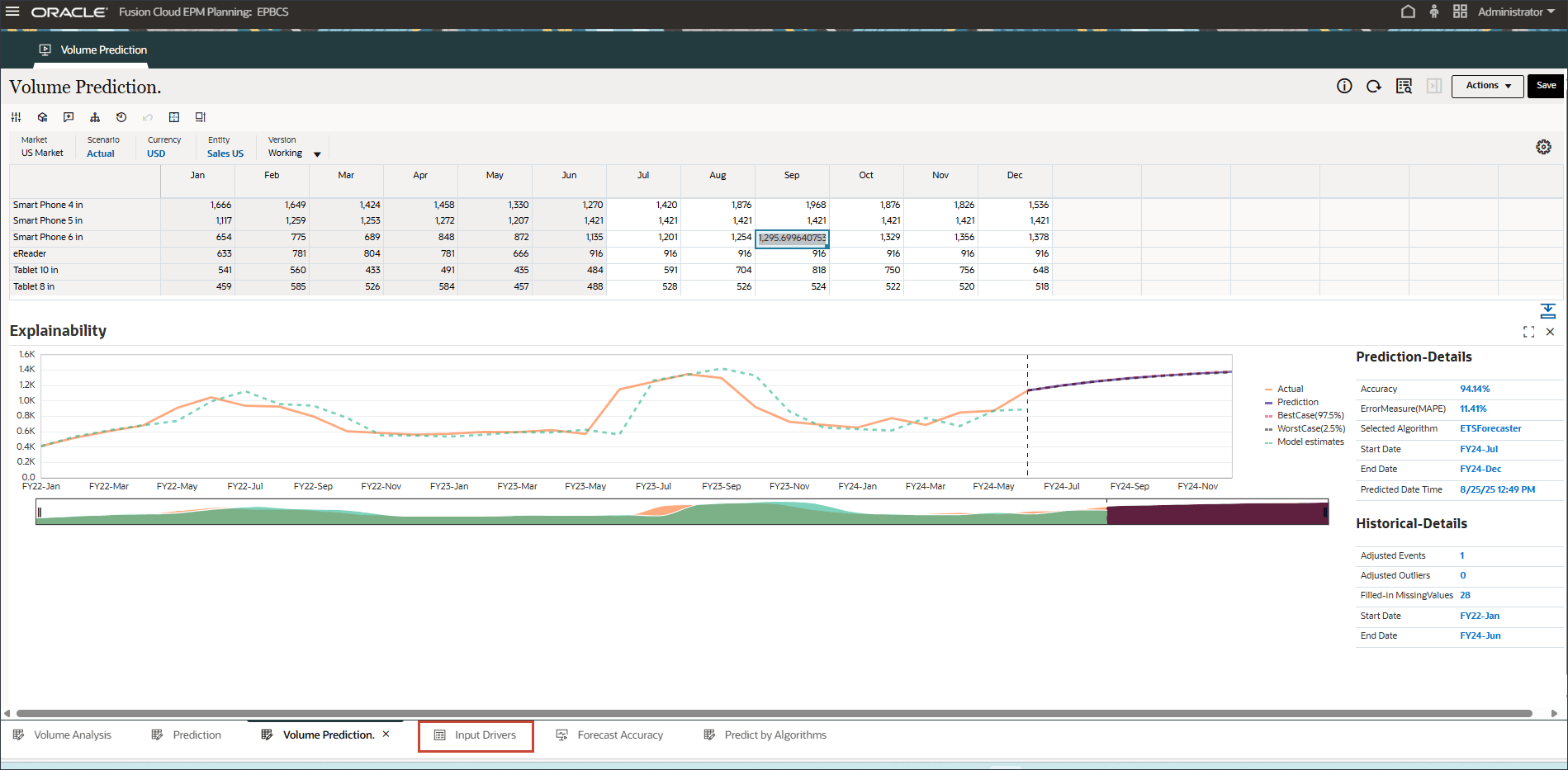
- Click Account, and select a driver such as Advertising and Promotion. Then enter and Save the updated values before running the Advanced Prediction job again.
- To run the Advanced Prediction job, follow the steps in the Running the Advanced Prediction Job section of this tutorial.
- Click
 (Home) to return to the Home page.
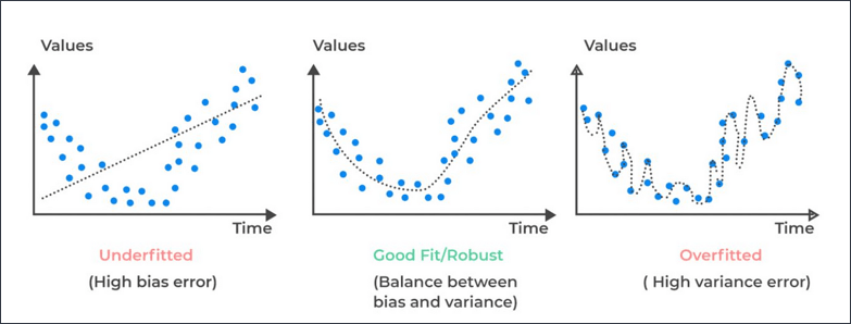
You can compare fitted values with historical actual data to see how well the prediction model was able to capture the variation in the provided data. The prediction was made using the trend for the future using the fitted value of historical data.

The dotted line/curve represents the fitted line, i.e. model’s estimates for historical data based on its learning of underlying logic/trends. If you compare the fitted values to the historical actual data you can see how well the model was able to capture the variation in the provided data.
Changing the Prediction Algorithm
In this section, you change the algorithm used to generate predictions. You make a copy of the advanced predictions job and modify the details to select a different prediction method.
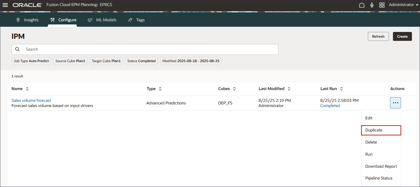
- On the home page, click IPM, then Configure.

- In the Sales volume forecast row, click
 (Actions), and select Duplicate.
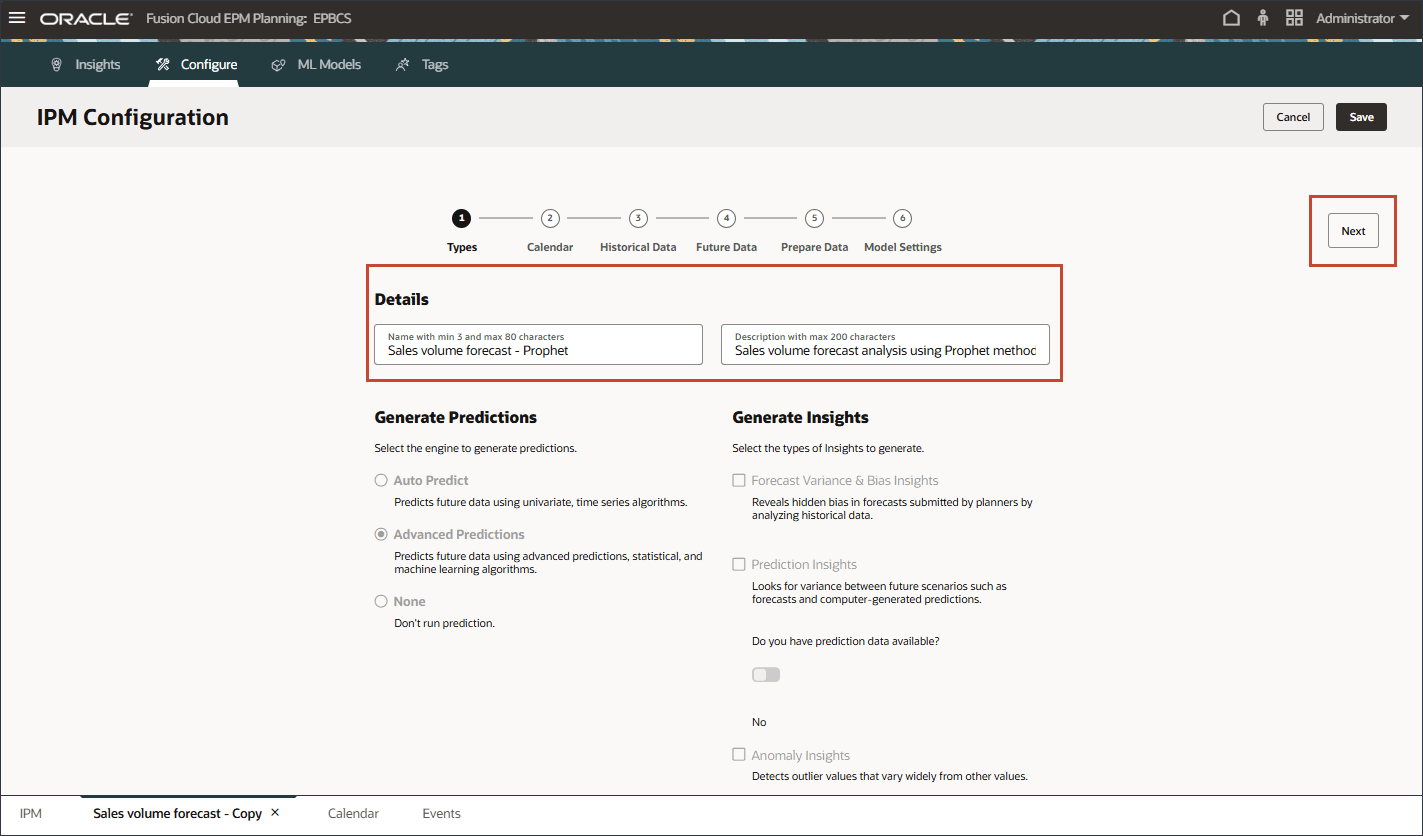
- To modify settings in the duplicate job, click Sales volume forecast - Copy.

- In Details, update the name to Sales volume forecast - Prophet, and the description to Sales volume forecast analysis using Prophet method, and click Next.
- Keep the calendar the same, and click Next.
- Keep the historical data slice the same, and click Next.
- For Future Data, in Define Model Scope, click Version.
- Select Prophet, and click OK.
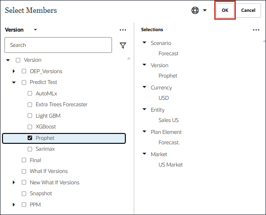
- Notice the updated Model Scope, and click Next.

- For the Prepare Data step, no changes are needed. Click Next.
- For the Model Settings step, in Select Algorithm, select Prophet.
Note:
The Prophet algorithm is not included in AutoML so you select Prophet to run Advanced Predictions using Prophet to see the results. The other algorithms are included within AutoML. - Ensure that for Forecast Error Metric, MAPE is selected.
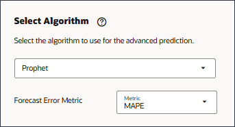
- For model estimates, best case, and worst case, change the version to Prophet.
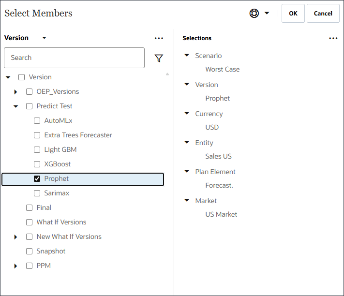
The version for model estimates, best case, and worst case are changed to Prophet.
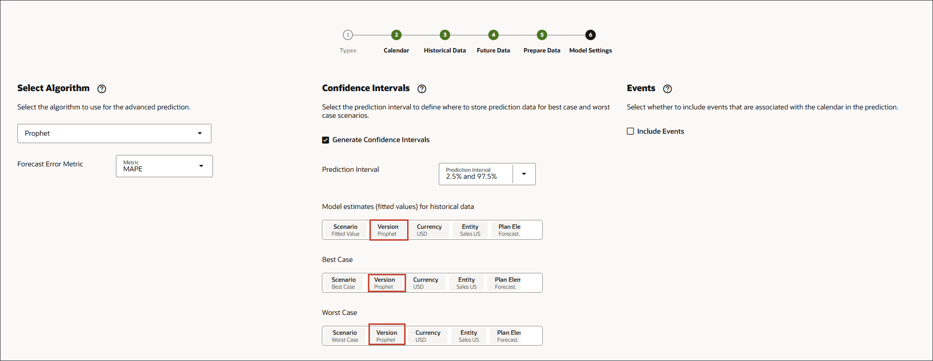
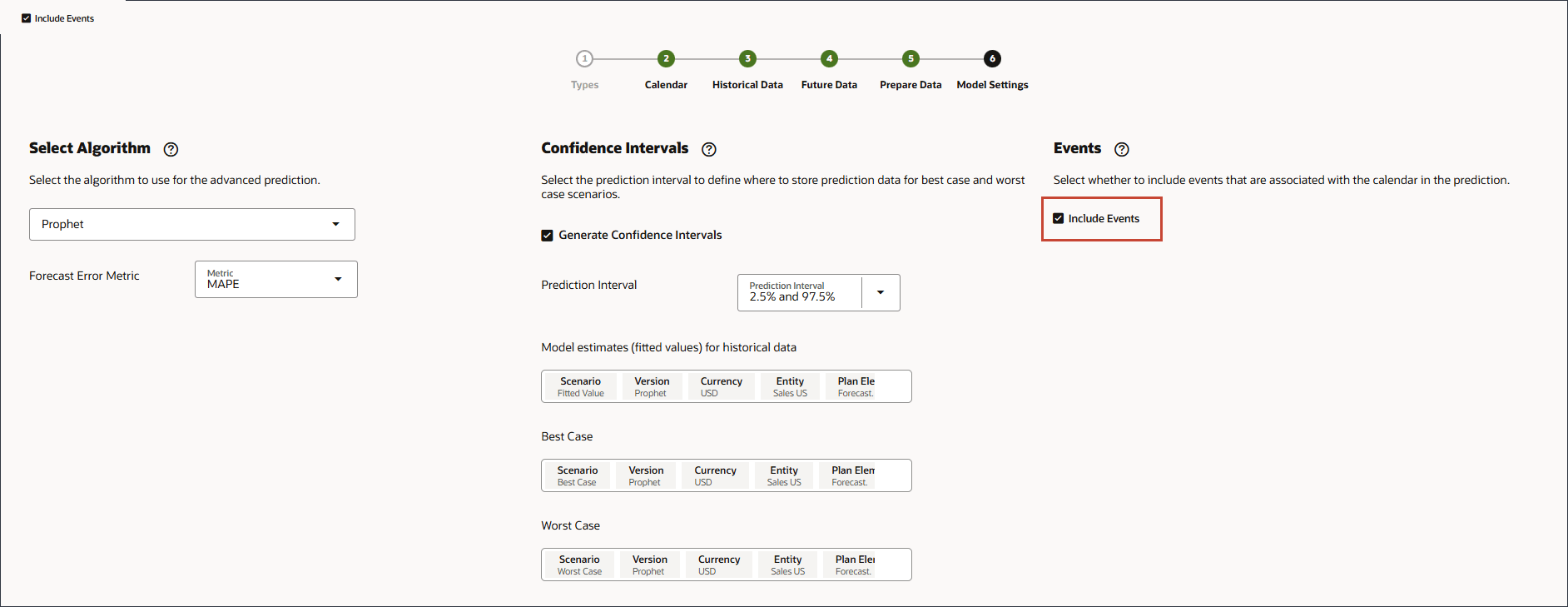
- Under Events, ensure that Include Events is selected, and click Save.
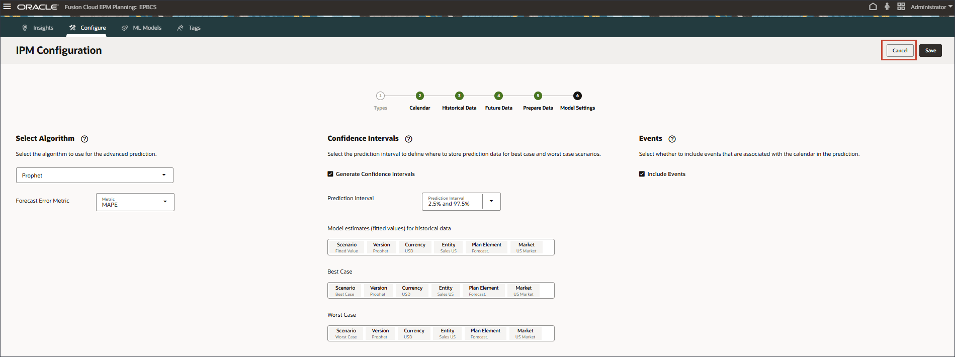
- Click Cancel.
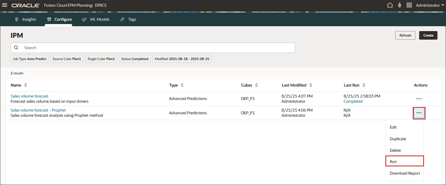
- For the Sales volume forecast - Prophet job, click
 (Actions), and select Run.
- Click Refresh until the job says it is completed.

Note:
The job takes a few moments to complete.The job is completed.

- Click
 (Home) to return to the Home page.
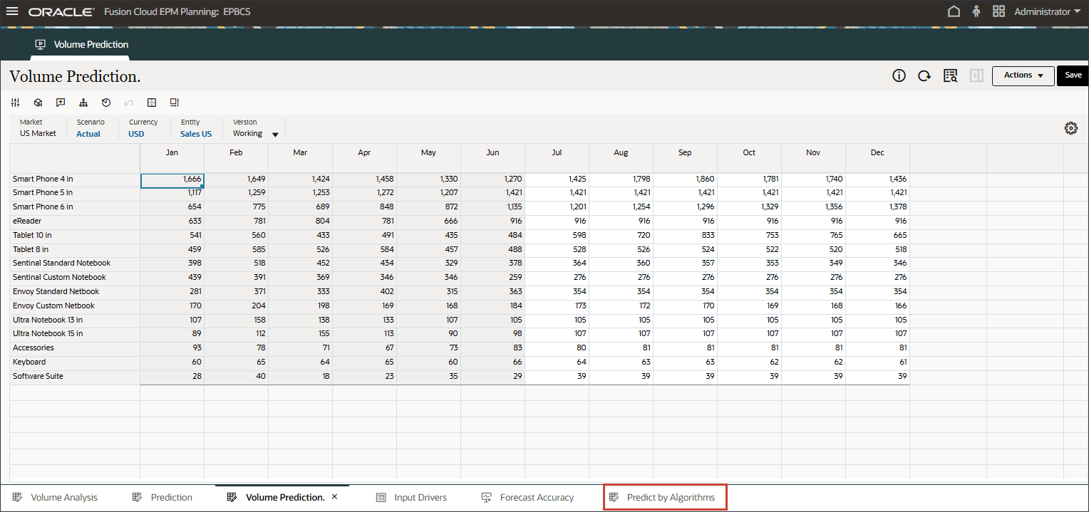
 - On the home page, click Advanced Predictions, and then Volume Prediction.

- On the bottom, select the Predict by Algorithms tab.
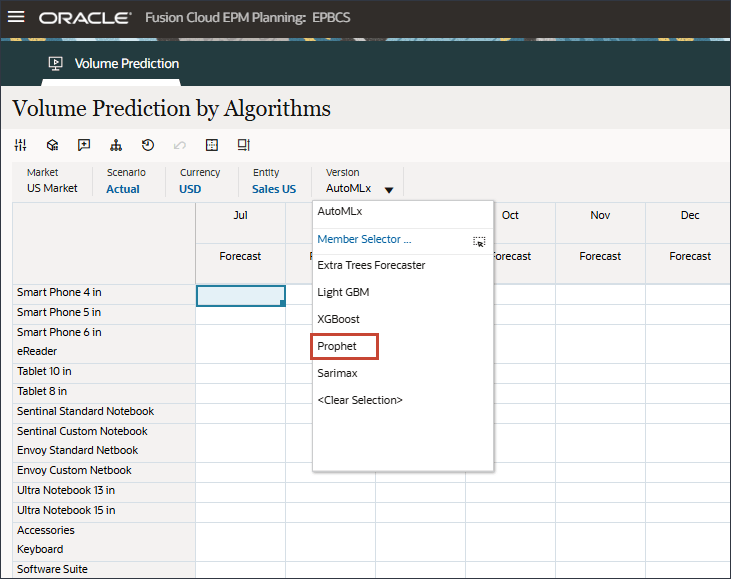
- For Version, select Prophet.
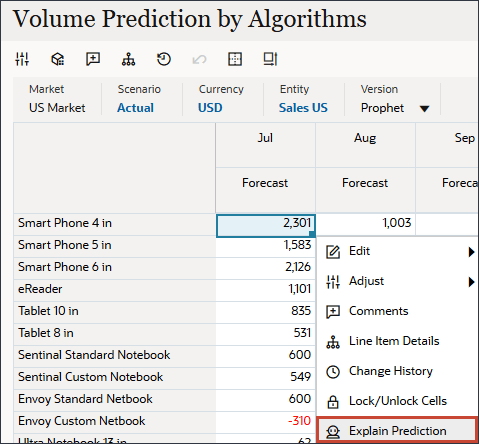
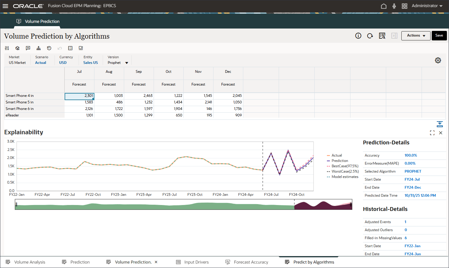
- Review the prediction by clicking Explain Prediction. Right-click a value such as Jul for Smart Phone 4 in, and select Explain Prediction.
Review the explainability. Notice that for some of the product series, Prophet has better accuracy.
Forecast Value Add
Forecast Value Add (FVA) is a metric used in forecasting to evaluate the effectiveness of the forecasting process by measuring the improvement (or decline) in accuracy due to changes in the forecasting method. FVA helps determine whether each step in the forecasting process adds value compared to a baseline, such as a naïve forecast or the previous forecast version.
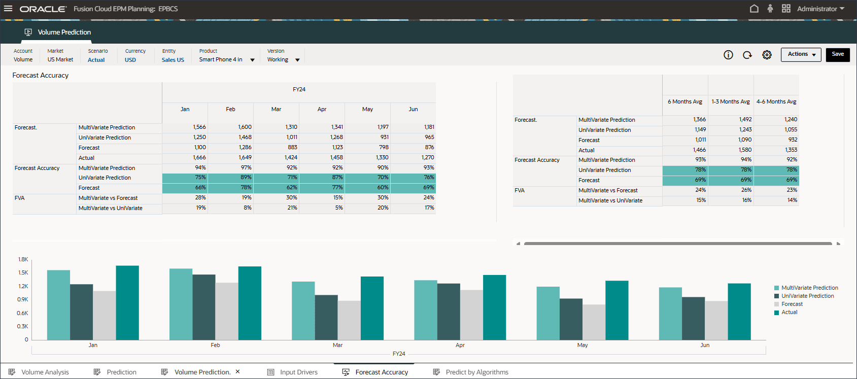
- On the bottom, click the Forecast Accuracy tab.
Testing is done to measure prediction accuracy for the period Jan-24 to Jun-24 where the actual data is already available. You can compare advanced prediction results (multi-variate prediction), univariate prediction, and forecast comparing those with the actual values to measure the accuracy of the forecast.
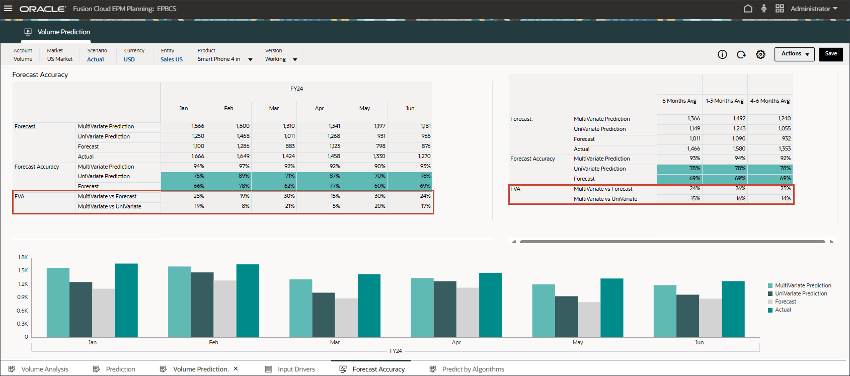
To calculate FVA, the accuracy of the adjusted forecast is compared to the accuracy of a baseline. If the adjusted forecast reduces errors compared to the baseline, then it has a positive FVA; if it increases errors, the FVA is negative. This metric helps forecasters focus on the steps that improve accuracy and eliminate non-value-adding activities in the forecasting process.
- Review forecast value add for advanced predictions (ML) to see that it is much better compared to the forecast and univariate prediction results.
- Review the bar chart which compares the Advanced Prediction results vs univariate predictions and forecast scenarios.
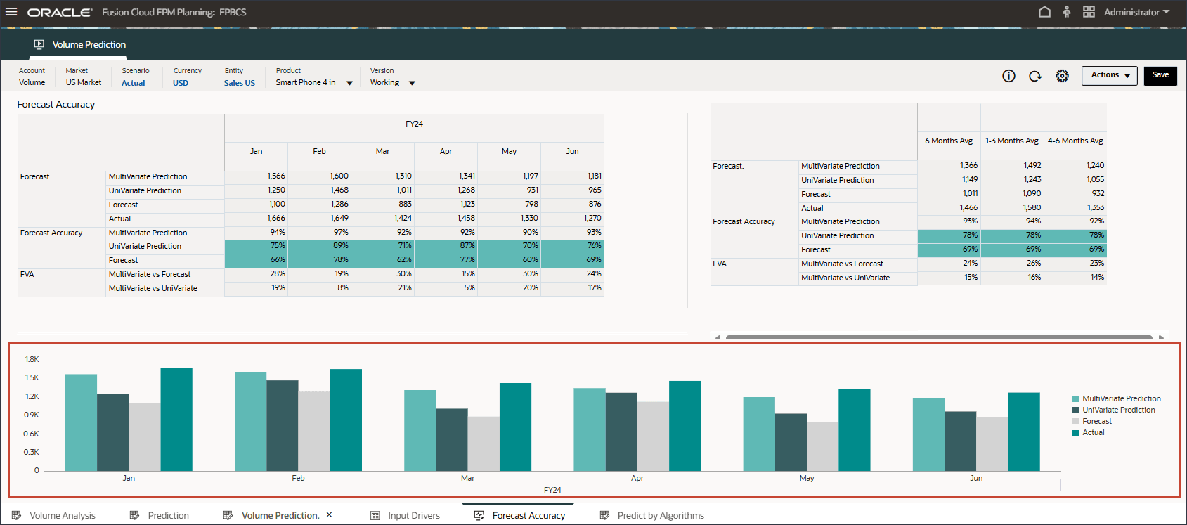
Advanced predictions using ML is closer to the actual results thereby increasing the confidence level for planners to use the Advanced Prediction method for future planning and forecasting.
Related Links
More Learning Resources
Explore other labs on docs.oracle.com/learn or access more free learning content on the Oracle Learning YouTube channel. Additionally, visit Oracle University to view training resources available.
For product documentation, visit Oracle Help Center.
Configuring and Reviewing Predictions with Advanced Predictions
G39822-05
March 2026