Planning and Foreacasting Using Predictive Planning

Introduction

This hands-on tutorial covers the essential tasks for using predictive planning as part of your planning and forecasting cycle. The sections build on each other and should be completed sequentially.

Background

Use Predictive Planning to predict future performance based on your historical data. You can compare and validate plans and forecasts based on the predictions. For a more accurate and statistically-based forecast, you can copy the prediction values and paste them into a forecast scenario for your plan. Predictive Planning works with EPM Standard and EPM Enterprise applications for Custom and Module application types. For legacy applications, Predictive Planning works with Standard, Enterprise, and Reporting application types. Predictive Planning is not available in FreeForm applications.

Prerequisites

Cloud EPM Hands-on Tutorials may require you to import a snapshot into your Cloud EPM Enterprise Service instance. Before you can import a tutorial snapshot, you must request another Cloud EPM Enterprise Service instance or remove your current application and business process. The tutorial snapshot will not import over your existing application or business process, nor will it automatically replace or restore the application or business process you are currently working with.

Before starting this tutorial, you must:

Have Service Administrator access to a Cloud EPM Enterprise Service instance.
Have the Planning sample application (Vision) created in your instance.

Adjusting User Variables

In this section, you will be adding values to the Product Family user variable.

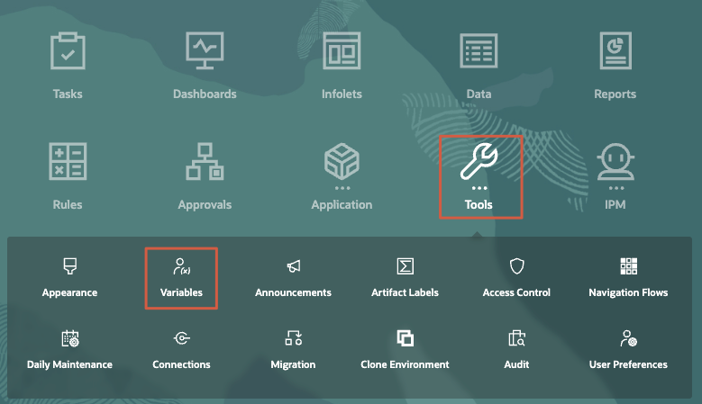
On the home page, click Tools, then User Variables.
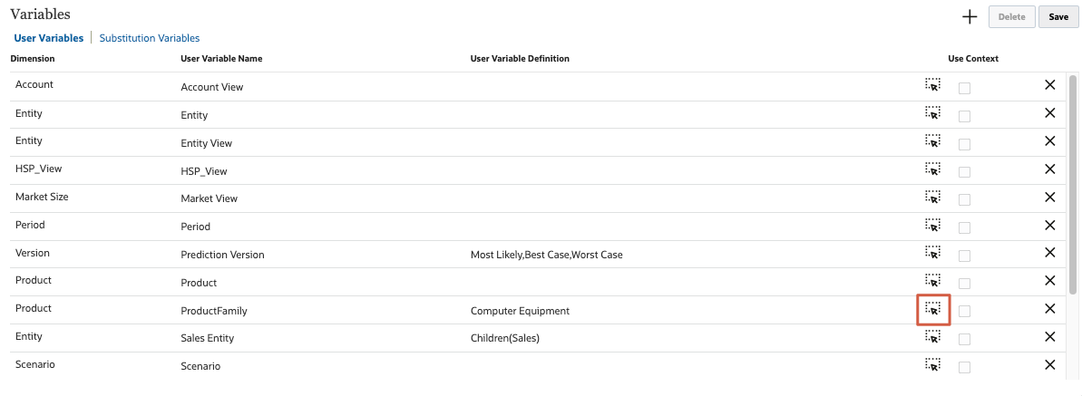
In User Variables, for ProductFamily, click (Member Selector).
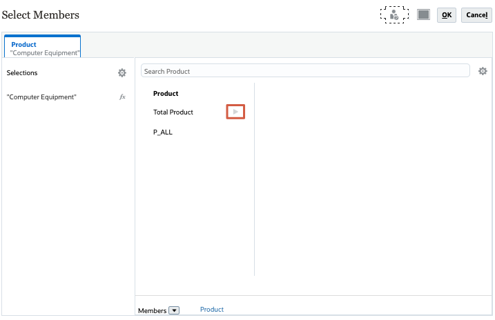
In Select Members, click the arrow next to Total Product.
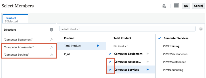
Under Total Product, select Computer Accessories and Computer Services.
When selected, the members are added to the Selections list on the left.
Click OK.
Verify that Computer Accessories and Computer Services were added to ProductFamily, and then click Save.
At the information message, click OK.
Return to the home page. On the upper-right, click (Home).

Running Predictive Planning

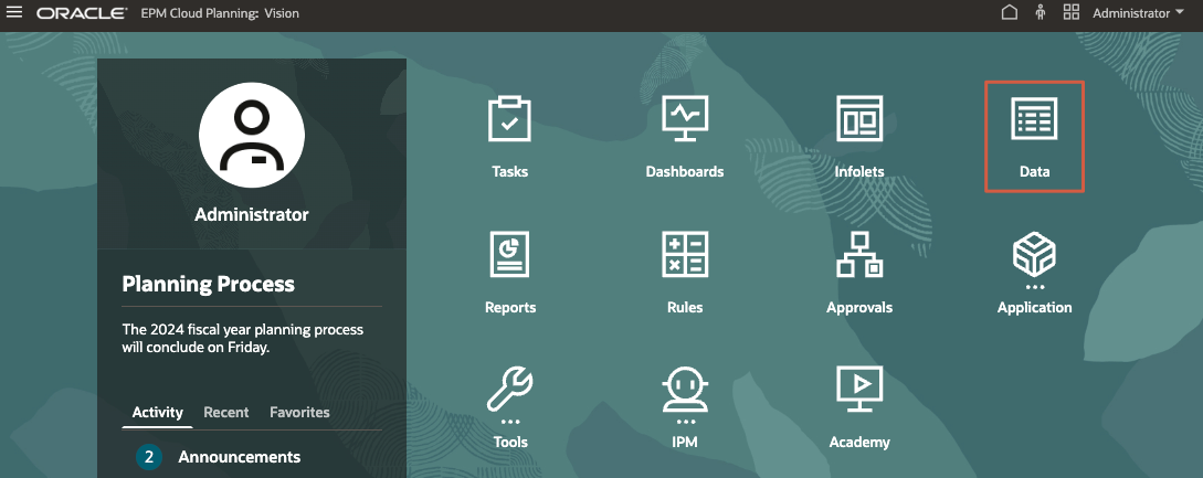
On the home page, click the Data card.
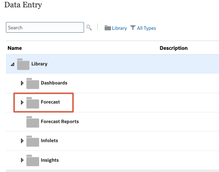
In Data Entry, under Library, expand Forecast.
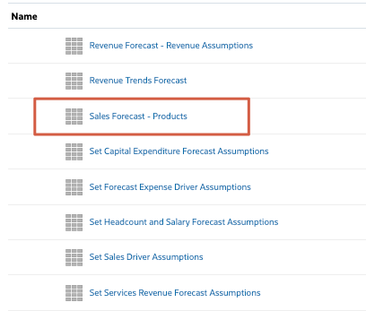
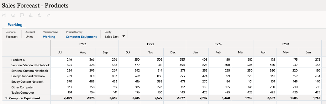
Scroll down and then click Sales Forecast - Products.
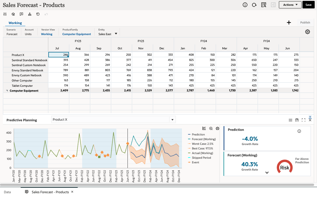
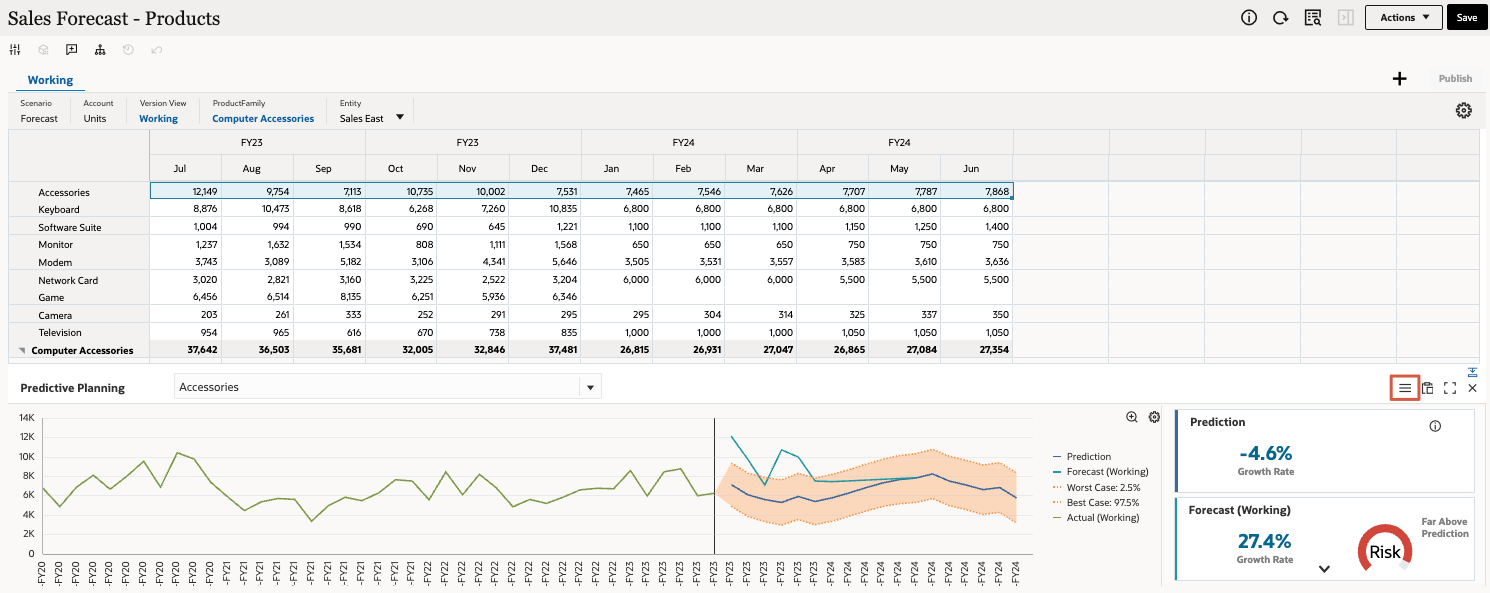
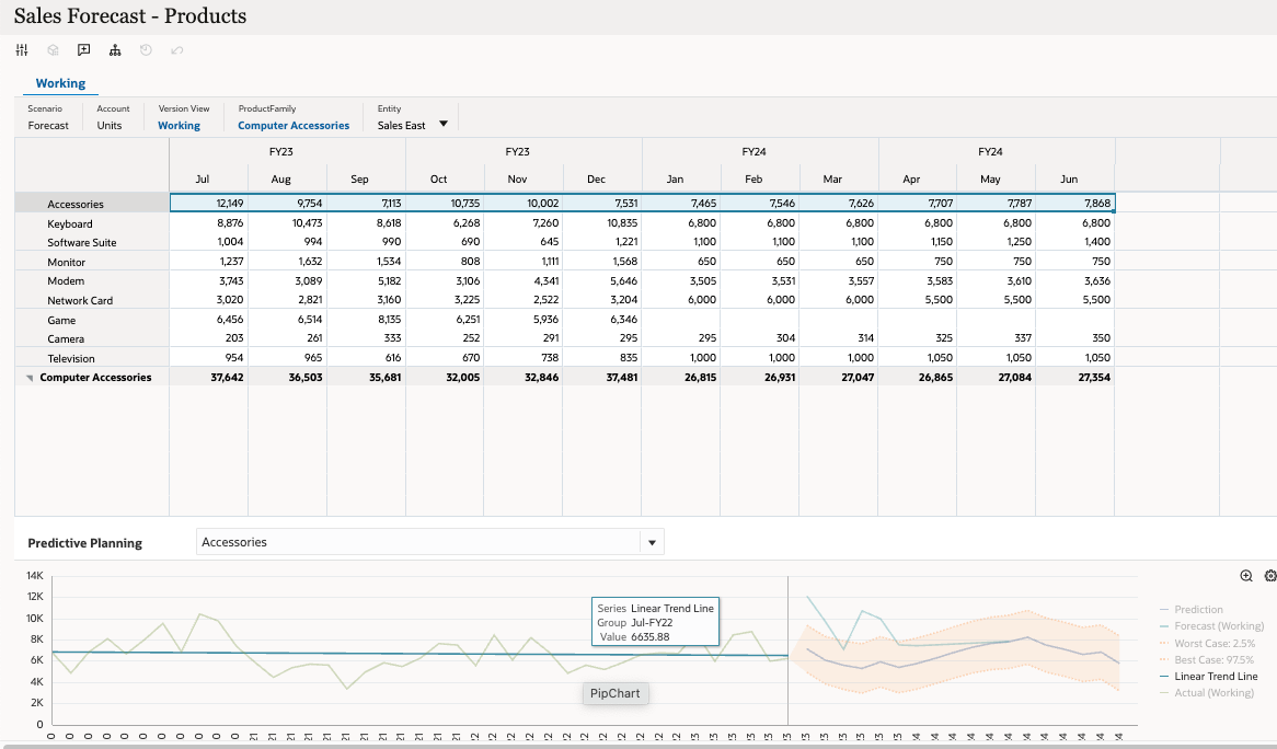
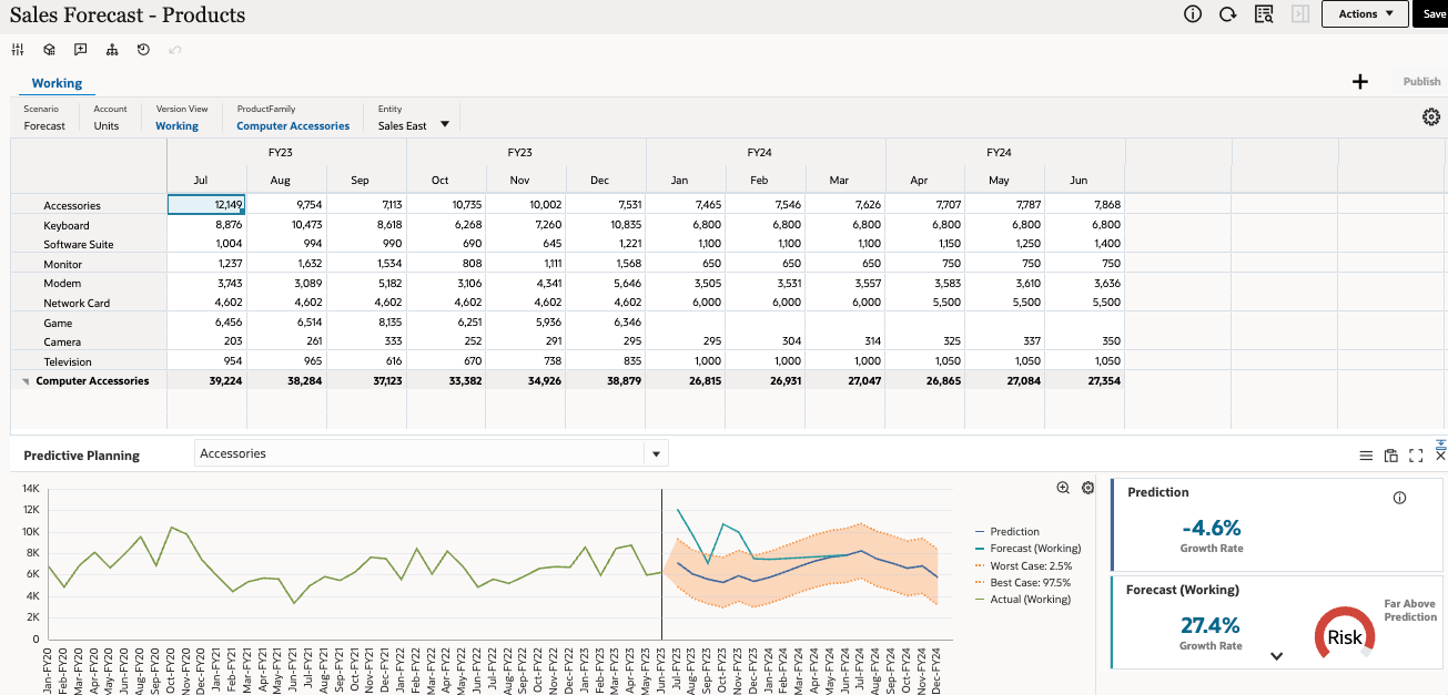
On the form, review sales forecast for each product under Computer Equipment for the upcoming planning time intervals.

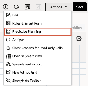
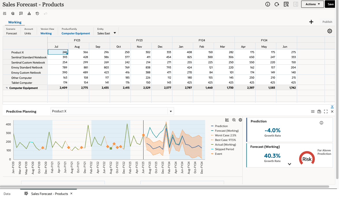
On the top right of the form, click Actions and select Predictive Planning.

When you run Predictive Planning, the system retrieves all the historical data for each member on the form. It then uses sophisticated time series forecasting techniques to predict the future performance for these members. The prediction results are displayed at the bottom of the form.
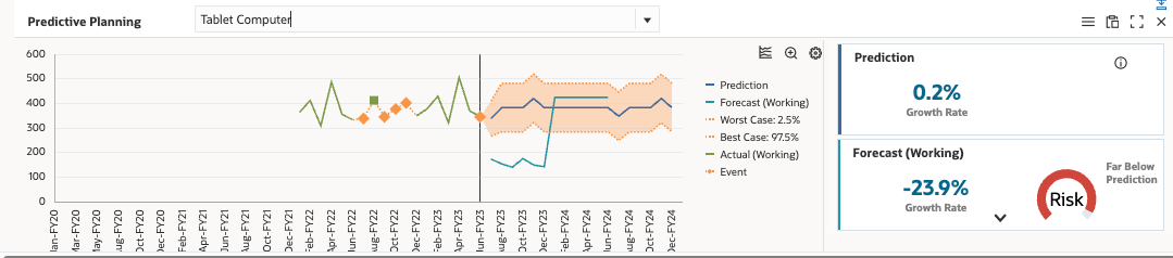
In the Predictive Planning section, use the down arrow to select Tablet Computer from the dropdown.
Review the prediction results for Tablet Computers.
The historical data for this product is shown as a green series on the left side of the chart. The base case prediction is shown in blue on the right. The prediction interval, which is bound by the Worst and Best cases, is shown as an orange band around the base case prediction.
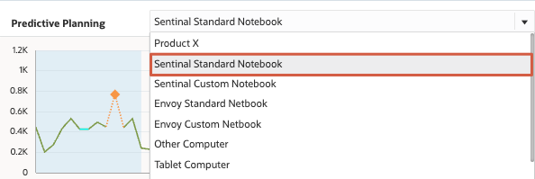
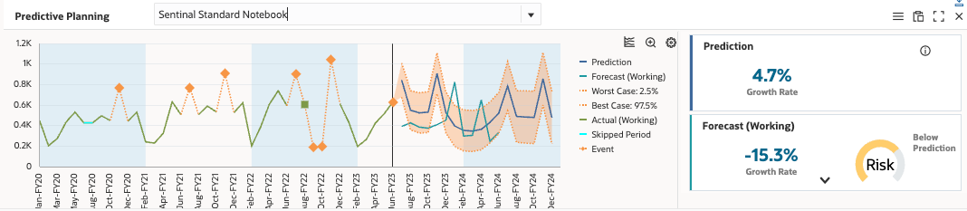
From the dropdown, select Sentinal Standard Notebook.
Compare the forecast against the statistical prediction. The Forecast scenario appears on the right side of the chart as a light green series.
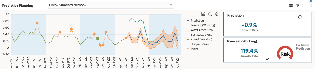
From the dropdown, select Envoy Standard Netbook.
Review the predictive results for this product.
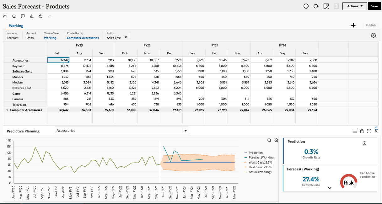
On the right side, view the informational boxes that contain key metrics for each series.
The Growth Rate metric allows the planner to quickly compare any two series. Based on the growth rate shown, the forecast is much more aggressive than the statistical prediction. The gauge to the right reflects the elevated risk for meeting the sales target for this product.

Understanding the Components of Predictive Planning

Predictive Planning provides a statistically-robust mechanism to help planners create and validate their forecasts using time series forecasting methods on historical data. Most forecasts created by users are based on gut feel or simple growth rates from previous years. However, Predictive Planning allows users to leverage time series forecasting techniques to produce more accurate forecasts.

When you open a form and run Predictive Planning, it produces the following results for each member on the form:

When you maximize the predictive results, the section is displayed with additional data:

Tip:

On upper right of the predictive results pane, click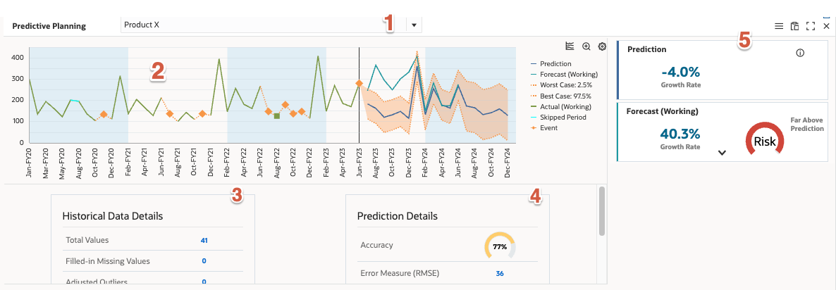

(Maximize) to expand the results view.

Member selection dropdown: Select any member on the form to display predictive planning results.
Chart area: Displays data for the selected member. Historical actual data is displayed on the left side of the chart. On the right side of the chart, partitioned by the vertical line, forecast and prediction data for the future time horizon is displayed. The chart area also contains data for the best case (optimistic) and worst case (pessimistic) scenarios.
Historical Data Details: Provides information on the historical data used for running the forecast algorithms. It includes the number of historical observations, missing values, outliers, presence of seasonality, etc.
Prediction Details: Provides details on the prediction output for the best-performing algorithm. Predictive Planning runs a set of time series forecasting algorithms on the historical data and picks the output from an algorithm that gives the best accuracy for the given member. It shows the name of the algorithm that has the highest accuracy compared to other algorithms and it provides RMSE and Accuracy metrics.
Information boxes: Provides a statistical summary of each series on the right side of the chart. It typically displays one box per series. The order of the boxes matches the order of the series in the legend.
- Growth Rate statistic is provided in each box as the key metric for comparing one series against another.
- Risk Gauge is added next to the growth rate to indicate the probability of the scenario occurring above or below the prediction.

How Predictive Planning Works

Predictive Planning is accessible from any form using the Actions menu.

Forecasting Algorithms

Two primary techniques of classic time-series forecasting are used in Predictive Planning:

Classic Non-seasonal Forecasting Methods — Estimate a trend by removing extreme data and reducing data randomness
Classic Seasonal Forecasting Methods — Combine forecasting data with an adjustment for seasonal behavior

Method	Seasonal	Best Use
Simple Moving Average	No	Volatile data with no trend or seasonality
Double Moving Average	No	Data with trend but no seasonality
Single Exponential Smoothing	No	Volatile data with no trend or seasonality
Double Exponential Smoothing	No	Data with a trend but no seasonality
Damped Trend Smoothing non-seasonal method	No	Data with a trend but no seasonality
Seasonal Additive	Yes	Data without trend but with seasonality that does not increase over time
Seasonal Multiplicative	Yes	Data without trend but with seasonality that increases or decreases over time.
Holt-Winters’ Additive	Yes	Data with trend and seasonality that does not increase over time
Holt-Winters’ Multiplicative	Yes	Data with trend and with seasonality that increase over time
Damped Trend Additive Seasonal Method	Yes	Data with a trend and seasonality
Damped Trend Multiplicative Seasonal Method	Yes	Data with a trend and with seasonality
ARIMA	No	Data with minimum of 40 historical data points, limited number of outliers and no seasonality
SARIMA	Yes	Data with minimum of 40 historical data points, limited number of outliers and seasonality

All of the non-seasonal forecasting methods are run against the data. If the data is detected as being seasonal, the seasonal forecasting methods are run against the data.

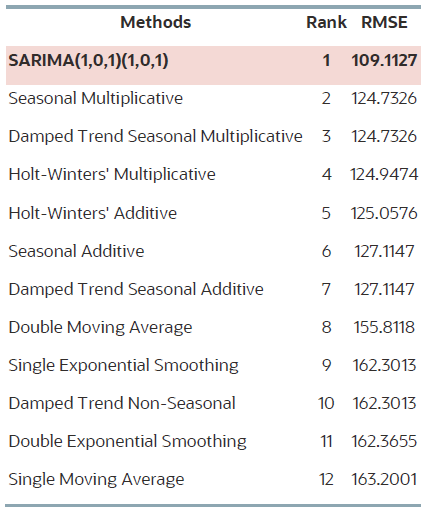
Selecting the Best-Performing Forecasting Model

The forecasting method with the lowest error measure (RMSE) is used to forecast the data. RMSE (root mean squared error) is an absolute error measure that squares the deviations to keep the positive and negative deviations from cancelling out one another. This measure also tends to exaggerate large errors, which can help eliminate methods with large errors. For instance, the forecasts from multiple algorithms are compared against each other based on the RMSE. The forecasting model with the lowest error, i.e. RMSE is chosen the best by default.

Example – Forecasting Non-Seasonal Data

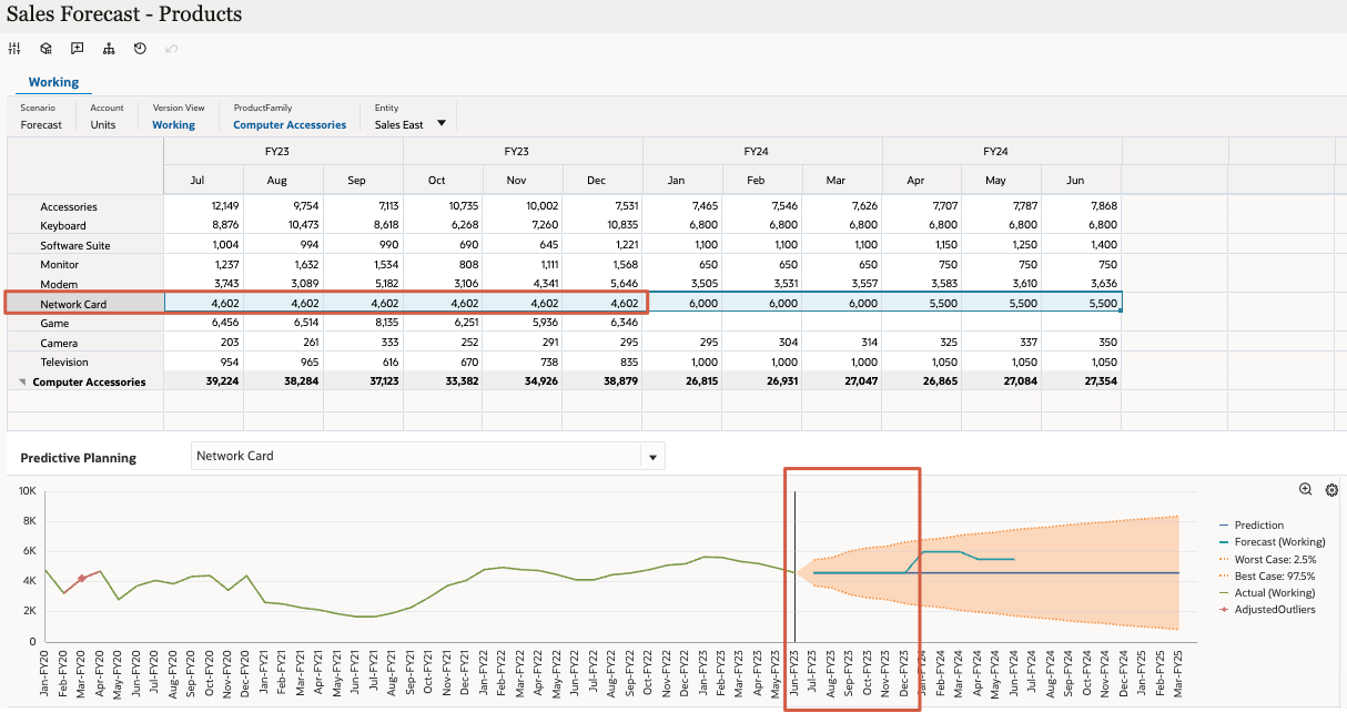
Here, we’re looking at the prediction results for Sales by product categories for the Sales East entity.

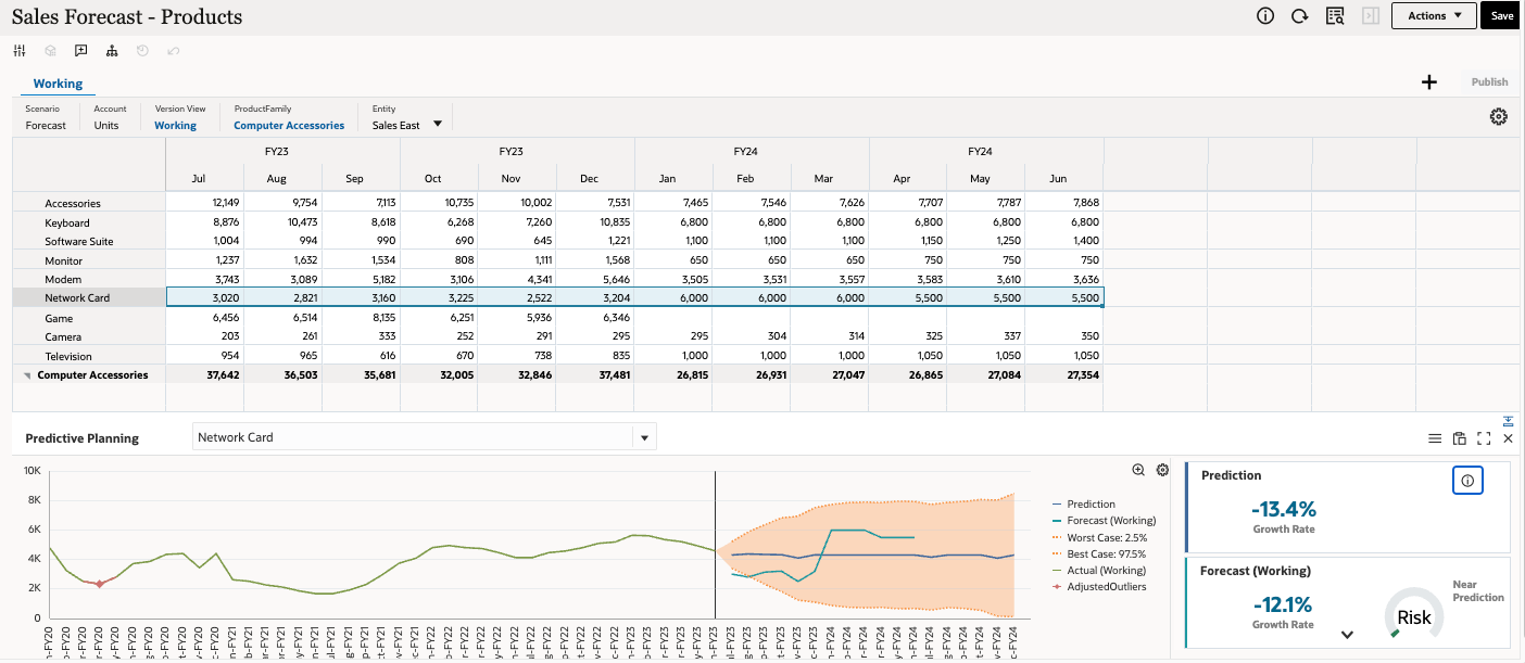
In this example, the product Network Card is selected. You can view the prediction results in the bottom panel. The historical data is shown as a green series on the left side of the chart. The base prediction is shown in blue on the right. The prediction interval, bound by the Worst and Best cases, is shown as an orange band around the base prediction. The historical data seems to be on an increasing trend and there is no obvious seasonality.

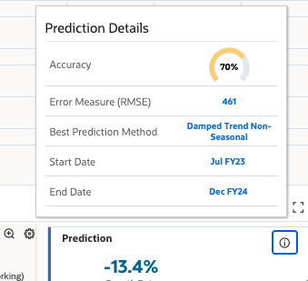
Tip:

To view more information about the prediction, click the information icon in the Prediction panel on the right.

The prediction output for this product category is from the Damped Trend Non-Seasonal method as it has the lowest error measure (RMSE) of 461. The prediction has an accuracy of 70% which is the likelihood of happening.

Example – Forecasting Seasonal Data

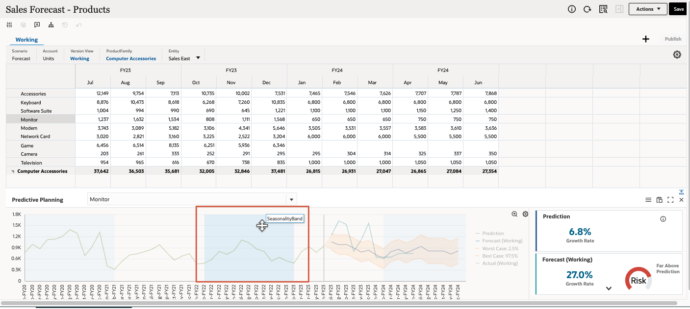
Here, we’re looking at the prediction results for the Monitor product in the Sales East entity.

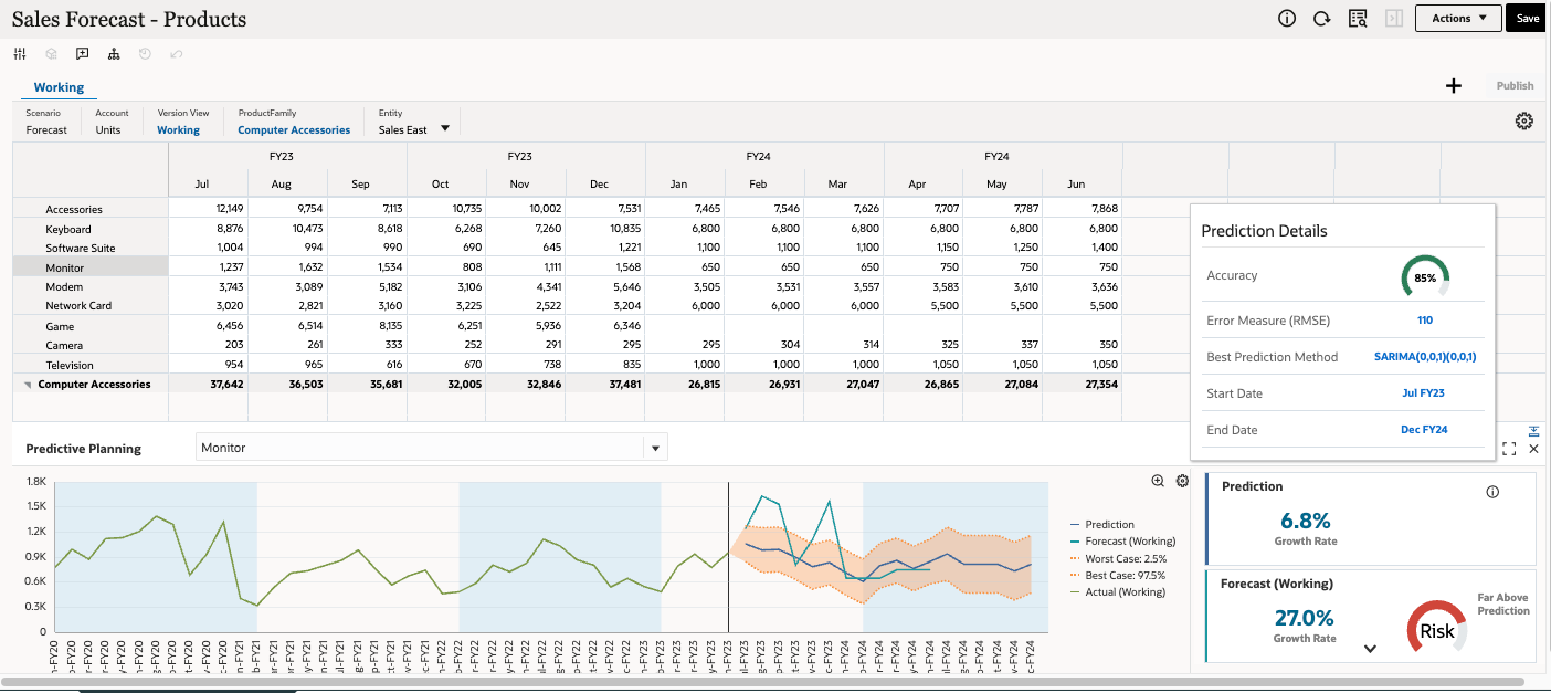
The historical sales for the Monitor product category have been seasonal as it hits the peak around August and December, and then sees lowest sales in January every year. The Seasonal ARIMA (SARIMA) method produces the most accurate results for this product category. Interestingly, the chart also captures the seasonality in the data as “seasonal bands”.

Example – Forecasting Seasonal Data Without Trend

View the prediction results for the Accessories product in the International Sales entity.

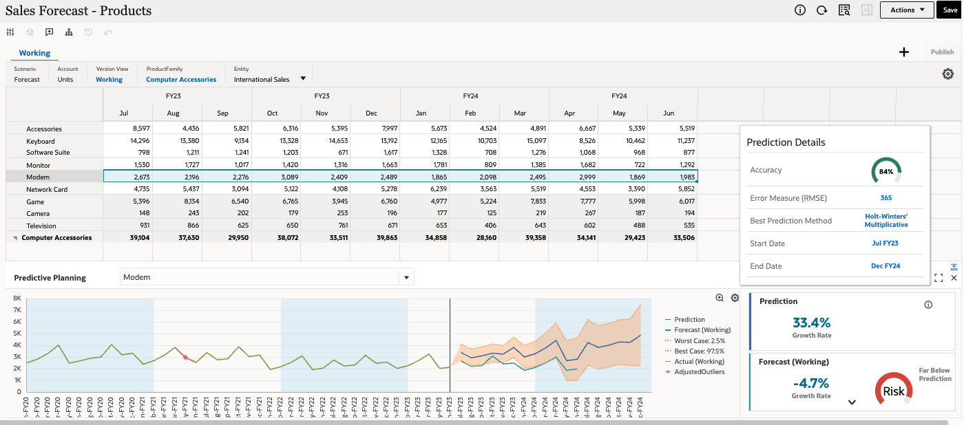
The historical actual sales show seasonality but no visible trend. The Holt-Winters' Multiplicative method gives the most accurate results for the given scenario.

Example – Forecasting Non-Seasonal Sales with Large Historical Data

Here are the prediction results for the Keyboard product in Sales East entity.

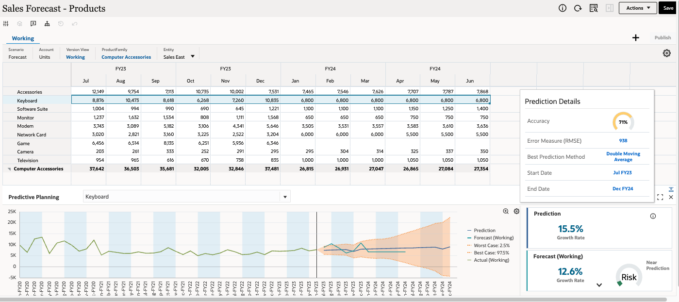
The historical actual sales show seasonal data. There is a good amount of historical data points and the Double Moving Average method gives the most accurate results for the given scenario.

Example – Forecasting Seasonal Sales with Large Historical Data

View the prediction results for the Other Computer product in the Sales East entity.

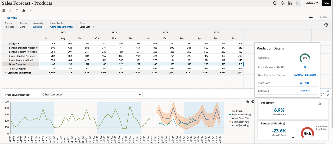
The historical actual sales show seasonality and there is also a clear increasing trend. Since it has a good amount of historical data (more than 40 data points), the Seasonal ARIMA (SARIMA) method gives the most accurate results for the given scenario.

Changing Settings in Predictive Planning

You can see the default settings used for a prediction. You can configure or customize these settings as needed.

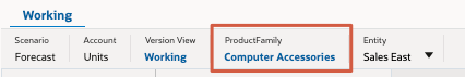
In the POV of Sales Forecast - Products, set ProductFamily to Computer Accessories.

Tip:
If your prediction results are not showing, close and reopen the form before re-running Predictive Planning.
Click Actions and select Predictive Planning.
In the Predictive Planning section, on the right, click (Settings).
In Settings, click the Chart View Settings tab.
In Chart View Settings, select Linear Trend Line - Past.
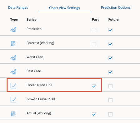
Click Apply.
The trend line for historical sales for the selected product is displayed in the chart.
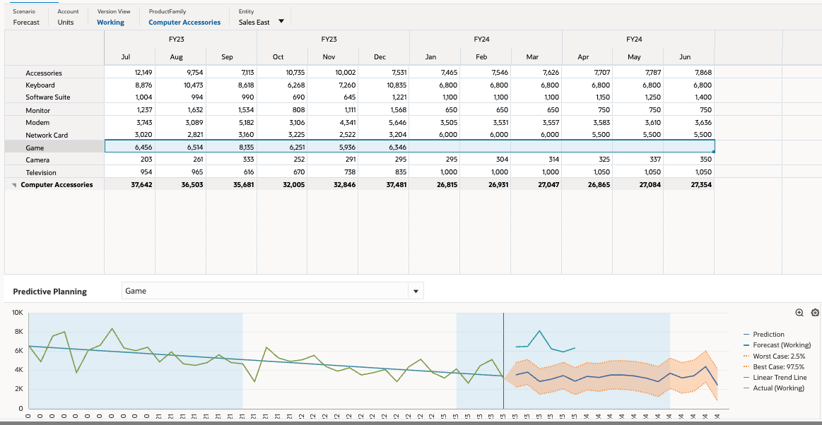
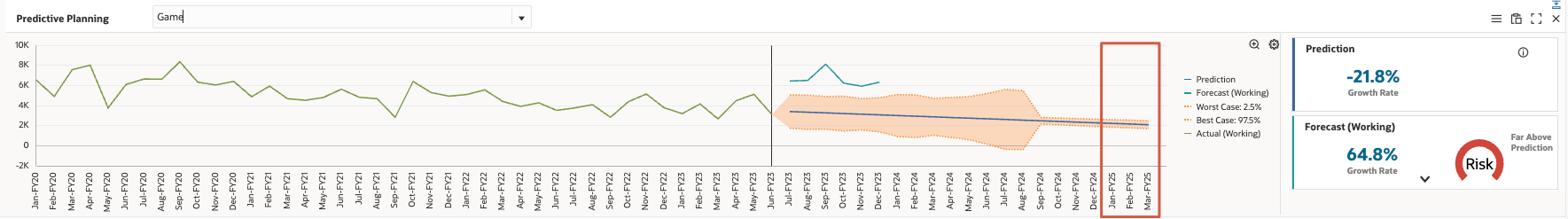
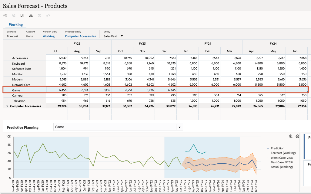
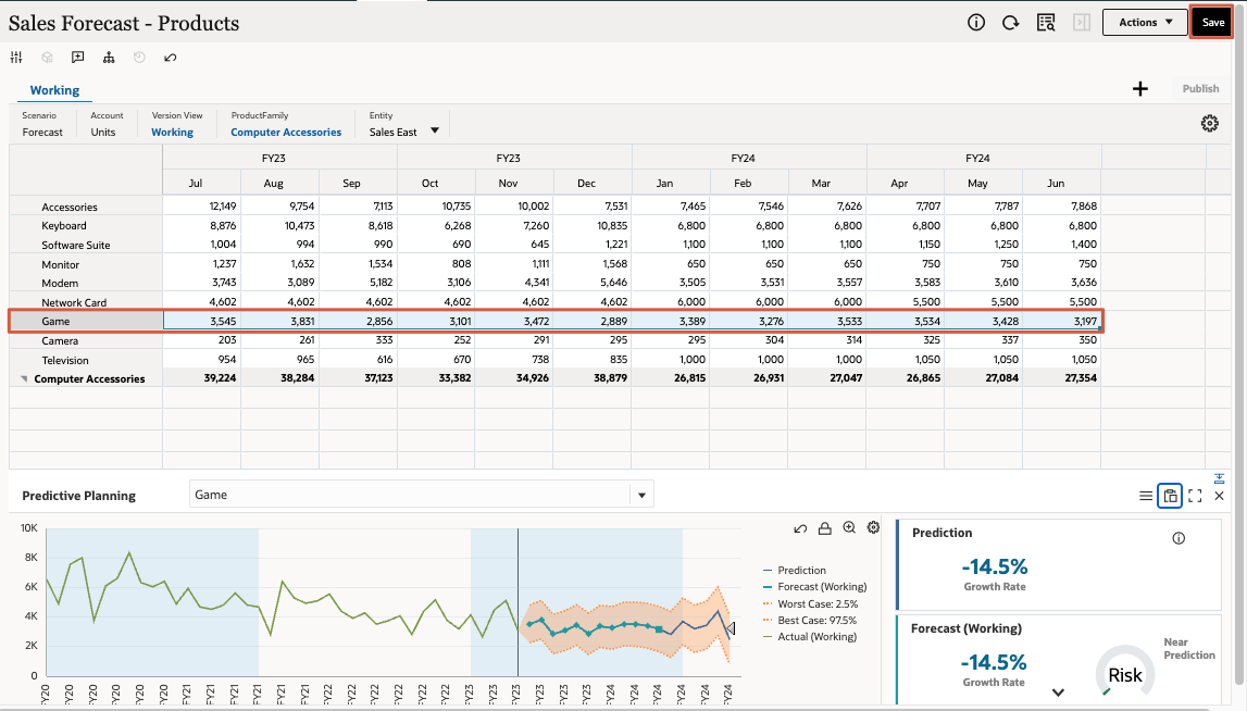
In Predictive Planning, select Game from the dropdown.
Notice that it has a declining trend in sales.
In the Predictive Planning section, on the right, click (Settings).
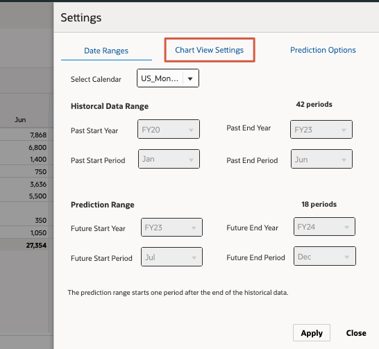
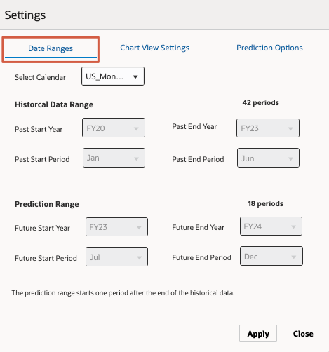
In Settings, make sure you are on the Date Ranges tab.
In the Select Calendar dropdown, remove the selection for the US_Monthly calendar and set it to --Select--.

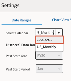
You can now modify date range selections.

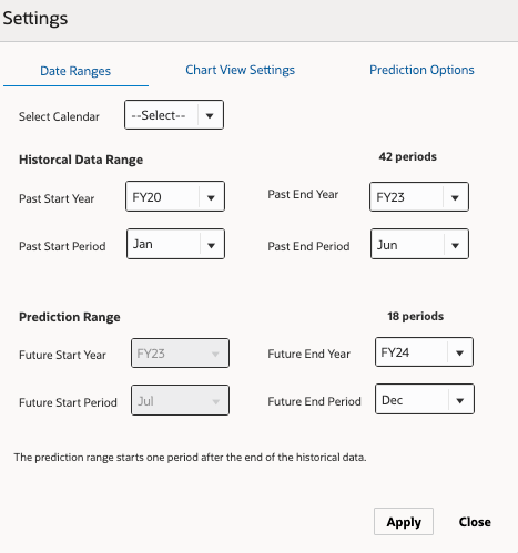
Tip:
When you select a calendar in Date Ranges, the historical data range and prediction range calendar options are taken from the options you defined for that calendar. To make changes, you must modify the calendar in the Calendar horizontal tab of the Configure card in the IPM cluster. If you do not select a calendar in Date Ranges, you can manually set the historical date range and prediction date range.
In Prediction Range, select the following dropdown options, and then click Apply:
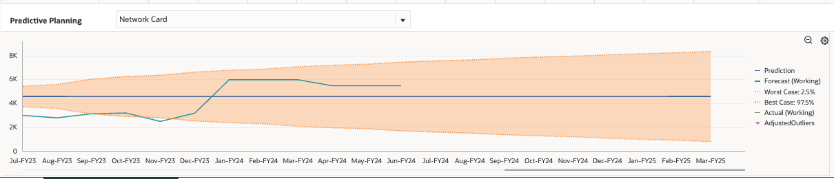
- Future End Year: FY25
- Future End Period: Mar
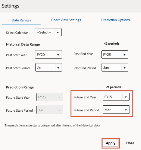
Notice the prediction/future time horizon is extended by 3 months, up to March 2025.

Adjusting the Forecast Based on Prediction

Once predictions have been calculated using Predictive Planning, compare the current forecast scenario with the predictions and make adjustments where required. This can be done by manually adjusting the forecast series by comparing it with the prediction.

In Sales Forecast - Products, make sure that Predictive Planning calculations were run.
Review the predictions for each member on the form.

In the grid, select the Network Card row to view the forecast against the statistical prediction for this product.

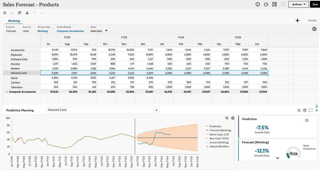
The prediction for Network Card product seems to be lower than the forecast scenario. We can adjust the forecast downward. We’ll first zoom into the prediction range and adjust the forecast manually by dragging the series on the chart.
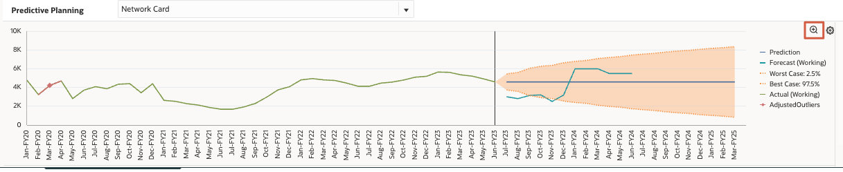
Click (Zoom In) to see the future start period portion of the chart in expanded view.

View the expanded results:

For the months with forecast values lower than the prediction values, adjust them in the series so that they align with each other. Click the Forecast (Working) item in the chart's legend to display the data points. Then, manually drag the line or data points in the chart. You can also manually adjust the values in the grid for July through December, and click Save.

Pasting the Prediction into the Forecast

After running predictions, you can compare the current forecast scenario with predictions and make adjustments to your data as needed. In the previous topic, you saw how this can be done by manually adjusting the forecast series by comparing it with the prediction. Alternatively, you can copy the prediction series and paste it to the forecast series.

In Sales Forecast - Products, make sure that Predictive Planning calculations were ran.
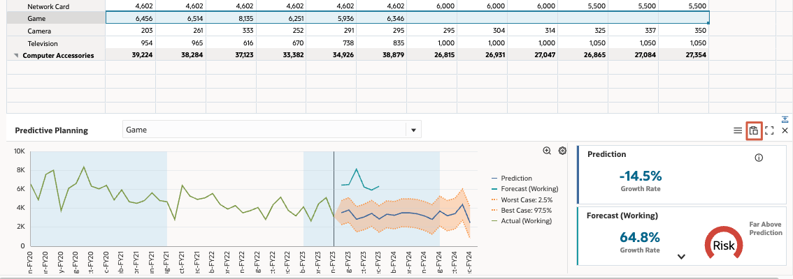
In the grid, select the Game row to view the forecast against the statistical prediction for this product.
In the top right of the Predictive Planning section, click (Paste).
In Paste Prediction, review and accept the default selections, and then click Apply.
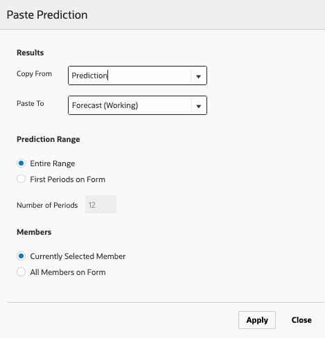
Review the prediction results pasted into the Forecast scenario for the Game product, and then click Save.
At the information message, click OK.

More Learning Resources

Explore other labs on docs.oracle.com/learn or access more free learning content on the Oracle Learning YouTube channel. Additionally, visit education.oracle.com/learning-explorer to become an Oracle Learning Explorer.

For product documentation, visit Oracle Help Center.

Title and Copyright Information