Analyzing Plan Data in Smart View

Before you Begin

This 40-minute tutorial shows you how to analyze plan data using ad hoc grid tasks in Smart View. The sections build on each other and should be completed sequentially.

Background

The seamless interchange between Web Ad Hoc Grids and Ad Hoc Grids in Smart View allow for flexible ways to work with and analyze data by focusing on data slices.

The redesigned ad hoc grid is available in Oracle EPM Cloud Planning, Tax Reporting, and Financial Consolidation and Close.

Perform ad hoc analysis with module-based, custom, and FreeForm Planning applications.

In this tutorial, you analyze plan data using ad hoc grid tasks in Smart View.

What Do You Need?

An EPM Cloud Service instance allows you to deploy and use one of the supported business processes. To deploy another business process, you must request another EPM Enterprise Cloud Service instance or remove the current business process.

You must have:

Service Administrator access to an EPM Enterprise Cloud Service instance.
The Planning sample application (Vision) created in your instance.
Microsoft Excel installed.
Smart View installed and configured to connect to your instance.

Tip:

You can download Smart View via the Downloads page in your instance or Oracle Technology Network.

About Ad Hoc Roles

Here are the roles you need to perform ad hoc tasks:

	Create	Modify	View	Perform Ad Hoc Operations	Save Ad Hoc Grid Definition	Submit Data
Service Administrator	✔	✔	✔	✔	✔	✔
Ad Hoc Grid Creator	✔	✔	✔	✔	✔	✔
Ad Hoc User		✔	✔	✔		✔
Ad Hoc Read Only User		✔	✔	✔

Note:

Learn more about role assignments in the Administering Access Control for Oracle Enterprise Performance Management Cloud documentation.

Connecting to Planning in Smart View

Connect to your instance and application before starting Ad Hoc Analysis.

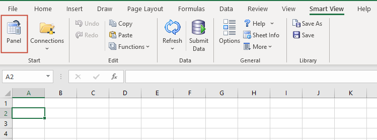
Launch Excel and make sure you have a blank worksheet open.
Select the Smart View ribbon and click Panel.
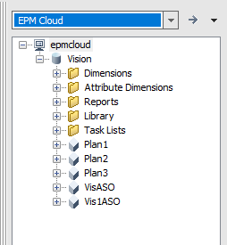
Connect to your EPM Cloud instance using Shared Connections, Private Connections, or Recently Used.
In this tutorial, a Shared Connection is used.
Expand the server node.
Expand Vision to display the application components.

Starting Ad Hoc Analysis

Open a form with the Ad hoc analysis option selected. This displays the Ad Hoc ribbon and enables ad hoc functionality.

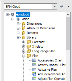
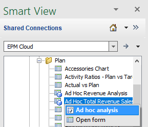
In the Smart View panel, under Vision, expand Library, and then Plan.
Locate and right-click Dept Income Statement - Plan and select Ad hoc analysis.

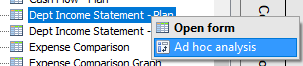
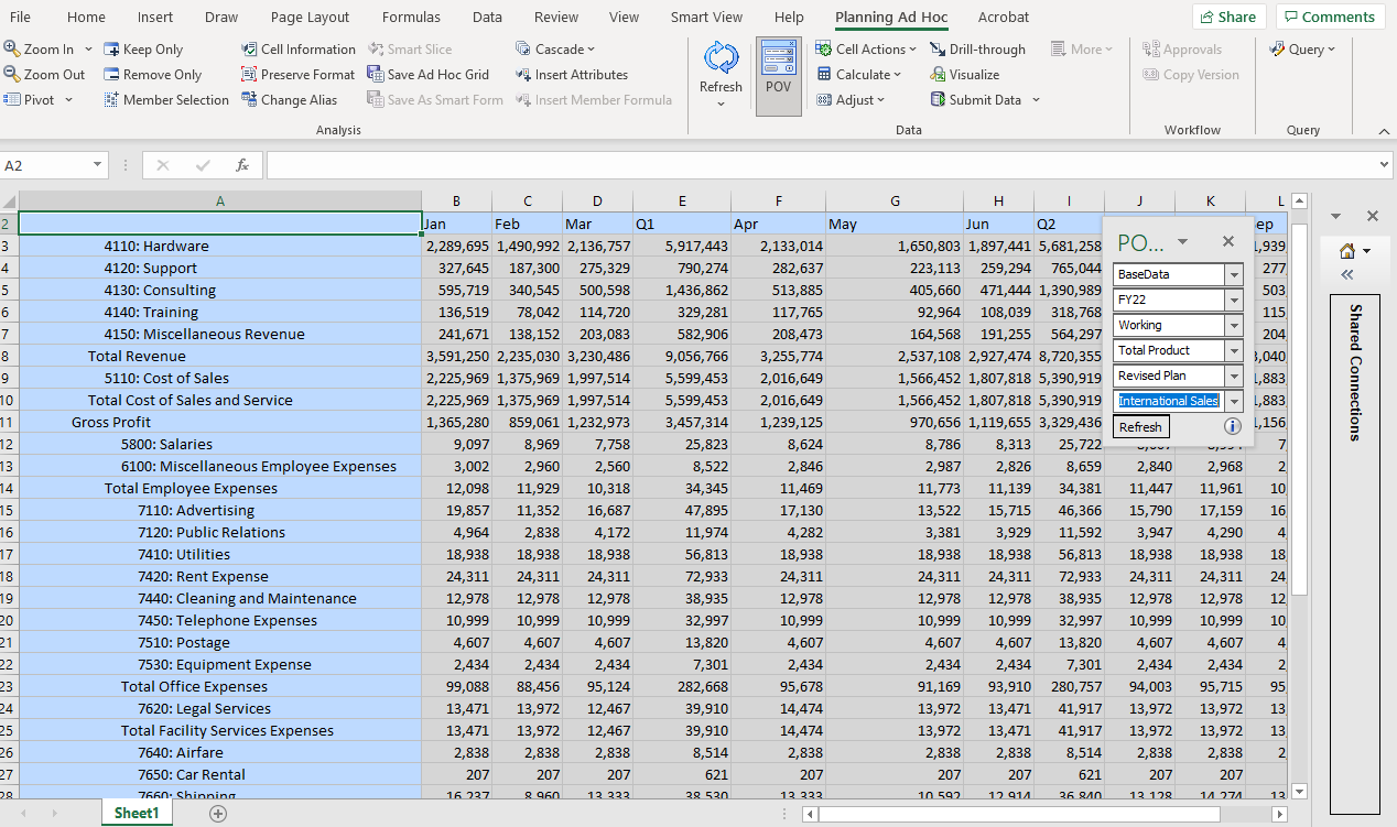
The form is opened in Ad Hoc mode, with the Planning Ad Hoc ribbon selected. The Planning Ad Hoc ribbon provides quick access to ad hoc analysis tasks.

Initially, you see the rows and columns from the form.

There is also a data point-of-view (POV) dialog where you can select members. You can dock or hide the POV.

Formatting Ad Hoc Grids

Formatting options control the textual display of members and data.

Formatting options are sheet-level options, which are specific to the worksheet for which they are set.

You can format your ad hoc grid according to options you select in Smart View Options - Formatting dialog.

Selecting Formatting Options

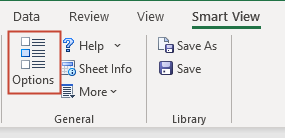
Select the Smart View ribbon.
Click Options.
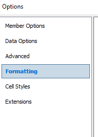
In Options, select Formatting.

Formatting options are displayed.
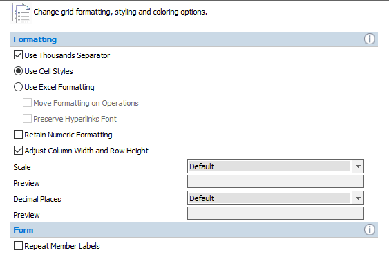
Review the following formatting options:
- Use Thousands Operator—Use a comma or other thousands separator in numerical data. Do not use # or $ as the thousands separator in Excel International Options.
- Use Cell Styles—Oracle Smart View for Office formatting consists of formatting selections made in the Cell Styles and Formatting tabs of the Options dialog box.
- Use Excel Formatting—Selec this option to use the built-in formatting options in Excel.
- Retain Numeric Formatting—When you drill down in dimensions, retains the Excel formatting you have set when selecting the Excel Home ribbon, then Format, and then Format Cells. For example, if you chose to display negative numbers in red, then negative values will be displayed in red as you drill down on any member. This option is only enabled when Use Cell Styles is selected.
- Adjust Column Width and Row height—Adjust column widths and row heights to fit cell contents automatically.
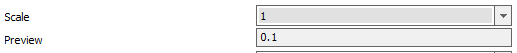
Optional: Accept the default or set the Scale to override the setting defined in the form definition. Choose a positive or negative scaling option.
The Preview in the next line displays a sample.

Here's an example:
Optional: Accept the default or specify the Decimal Places for the data values.
The Preview in the next line displays a sample.

Here's an example:
Optional: Select Repeat Member Labels to allow member names to appear on each row of data.
Review your selections and click OK.
On the Smart View ribbon, click Refresh to apply the formatting options to the grid.

Using Excel Formatting

If you use Excel formatting, your formatting selections, including conditional formatting, are applied and retained on the grid when you refresh or perform ad hoc operations.

When you use Excel formatting, Smart View does not:

Reformat cells based on your grid operations
Mark cells as dirty when you change data values

Smart View preserves the formatting on the worksheet between operations.

Using Excel formatting is generally preferable for highly formatted reports, and you must use Excel formatting for data sources whose application-specific colors are not supported by the Excel color palette.

On the Smart View ribbon, click Options.
In the left pane, select Formatting
Select Use Excel Formatting.
Optional: Select Move Formatting on Operations.
Optional: Select Preserve Hyperlinks Font.

Note:
If you select Excel Formatting, Retain Numeric Formatting is disabled.
Click OK.
On the Smart View Ribbon, click Refresh to apply the formatting options to the grid.

Using Cell Styles

You can specify formatting to indicate certain types of member and data cells. Because cells may belong to more than one type (for example, a member cell can be both parent and child), you can also set the order of precedence for how cell styles are applied.

Cell style options are global options, which apply to the entire current workbook, including any new worksheets added to the current workbook, and to any workbooks and worksheets that are created subsequently. Changes to global option settings become the default for all existing and new Microsoft Office documents.

Selecting Apply to All Worksheets or Save as Default Options are optional.

On the Smart View ribbon, click Options.
In the left pane, select Formatting.
Select Use Cell Styles.
select Cell Styles.
Cell Styles control the display of certain types of member and data cells.
Expand Planning and Common.
Expand Member cells and Data cells.
Because cells may belong to more than one type—a member cell can be both parent and child, for example—you can also set the order of precedence for how cell styles are applied.
Select an object type under Member cells, Data cells, or Common.
Click Properties and select an option: Font, Background, or Border.
- If you selected Font, make your font selections on the Font dialog box and click OK.
- If you selected Background, select a color and click OK.
- If you selected Border, select a color and click OK.
Collapse Planning.
Click OK.
On the Smart View Ribbon, click Refresh to apply the formatting options to the grid.

Setting Data Options

On the Smart View ribbon, click Options.
In the left pane, select Data Options.
Set options to control the display of data cells.

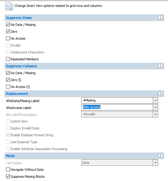
Data options are sheet-level options, which are specific to the worksheet for which they are set.
Click OK.
On the Smart View Ribbon, click Refresh to apply the data options to the grid.

Setting Member Options

Member Options control the display of member cells.

Member options are sheet-level options, which are specific to the worksheet for which they are set.

On the Smart View ribbon, click Options.
In the left pane, select Member Options.
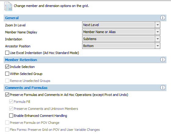
To preserve Excel formulas in ad hoc grid, make sure that Preserve Formulas and Comments in Ad Hoc Operations (except Pivot and Undo) is selected.
Click OK.

Performing Ad Hoc Analysis

Perform ad hoc tasks by selecting members, using functions, and performing a variety of operations, including formatting, to design and build your reports.

Note:

Learn how you can create multiple ad hoc grids on one worksheet by viewing the Setting Up Multiple Grids in Smart View tutorial.

Keeping and Removing Members

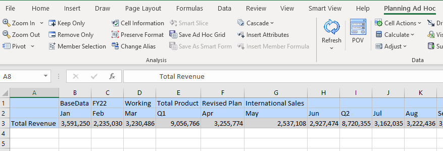
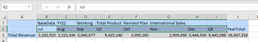
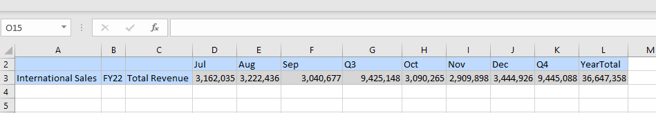
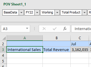
You can customize your ad hoc grid by keeping or removing selected members. In this example, you keep the Total Revenue member and remove the first two quarters of the year.

Select the Planning Ad Hoc ribbon.
In the grid, select Total Revenue.
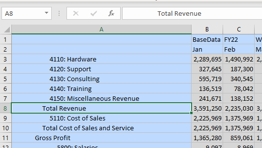
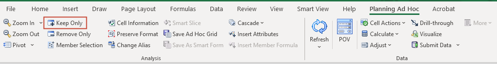
On the Planning Ad Hoc ribbon, click Keep Only.

The grid is updated. Only the current selected member is displayed.
In the grid, select Jan, Feb, Mar, Q1, Apr, May, Jun and Q2.
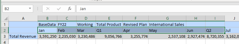
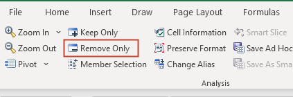
On the Planning Ad Hoc ribbon, click Remove Only.

The grid is updated. Only the current selected member is displayed.

Pivoting Members

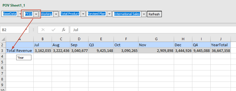
You can pivot dimensions to the POV, columns, or rows. The available choices depend on which axis the dimension is located before you pivot it.

Pivot a dimension from the POV to the rows. From the POV, click and drag the Year dimension (FY22) to the rows.
Pivot a dimension from the POV to the columns. From the POV, click and drag the Entity dimension (International Sales) to the columns.
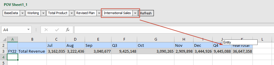
Pivot a dimension that is currently in the rows or columns. In the grid, click International Sales.
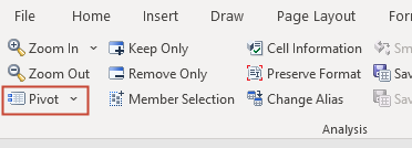
On the Planning Ad Hoc ribbon, click Pivot.

When you select Pivot, if the dimension was in the column, your action moves it to the row. Similarly, if the dimension is in the row, your action moves it to the column.

When you pivot a member, the other members in its dimension are also pivoted.

Note:
You cannot pivot the last dimension in a row or column.
In the grid, click the Year dimension (FY22).
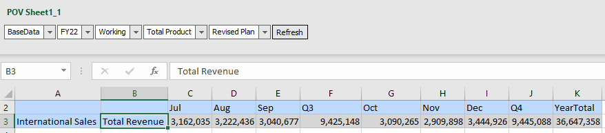
On the Planning Ad Hoc ribbon, click the down-arrow next to Pivot to display options, and select Pivot To POV.

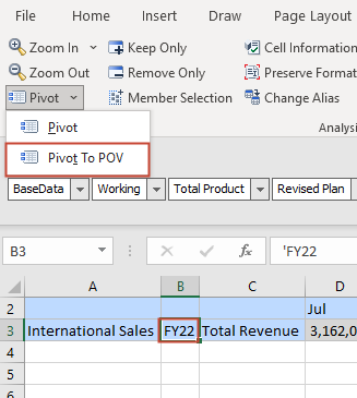
Pivot dimensions based on your reporting requirements. For example, if you are analyzing only one year of data, you can pivot the Year dimension back to the POV.

Selecting Members

You can select members for dimensions in your ad hoc grid by using the Member Selection dialog.

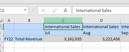
Select members for Entity. In the grid, select the Entity dimension (International Sales).
On the Planning Ad hoc ribbon, click Member Selection.
Expand Total Entity, then Total Department, and then Sales.
Select International Sales, Sales East, and Sales West, and then click Add.
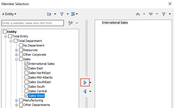
Click OK.
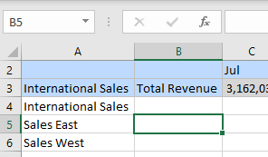
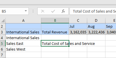
Select members for Account. In the grid, select the Account dimension cell for Sales East.
On the Planning Ad hoc ribbon, click Member Selection.
In Member Selection, use the search feature to find members. In the Search field, type Total Cost of Sales and Service and press <Enter>.
Select Total Cost of Sales and Service and click Add.
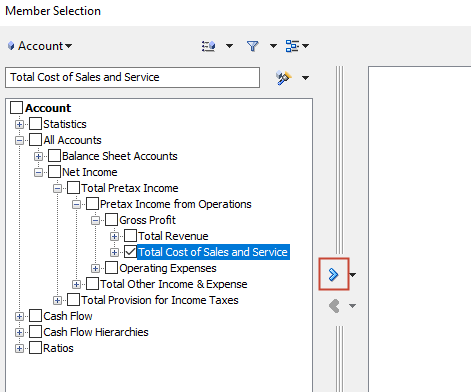
Click OK.
The grid is updated with member selections.
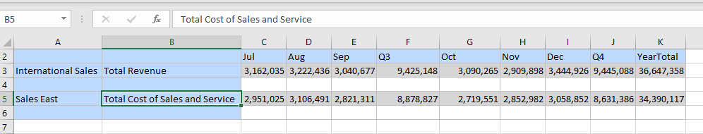
On the Planning Ad Hoc ribbon, click Refresh.
The grid displays data for the selected members.
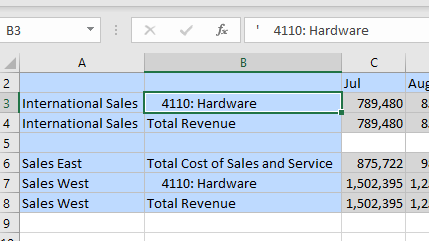
In the grid, below Sales East, enter Sales West as the entity and Total Revenue as the account.
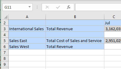
On the Planning Ad Hoc ribbon, click Refresh.
The grid displays data for the selected members.
Select members for dimensions on the POV. In the POV, click the Product dropdown list and select the ellipsis.
In Member Selection, expand Total Product, then select Computer Equipment.
Click the down arrow next to Add and select Descendants Inclusive.
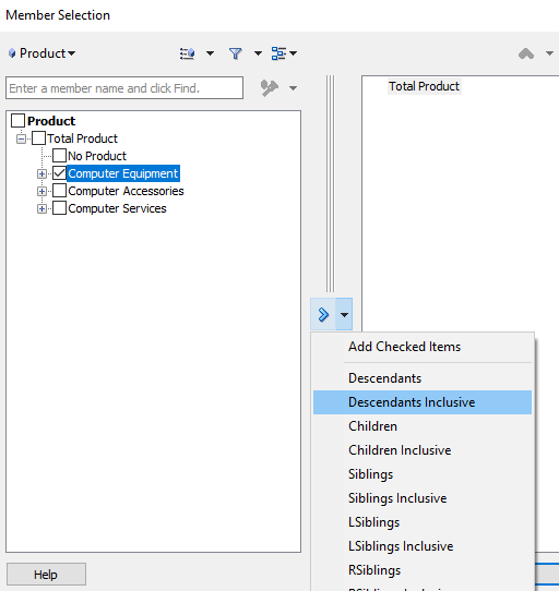
Click OK.
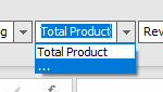
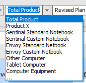
In the POV, click the Product dropdown list to view the updated list of members.
Select Computer Equipment and click Refresh.
The ad hoc grid displays data based on your member selections.

Tip:

When performing ad hoc analysis, you can use the Insert Attributes option from the Planning Ad Hoc ribbon to insert attribute dimensions or members on the worksheet.

Zooming In and Out Member Levels

You can zoom in and out to display data for different levels in the dimension hierarchy.

In the grid, select the Total Revenue account member for International Sales.
On the Planning Ad hoc ribbon, click the down arrow for Zoom In to display options.
Select Next Level.
The updated grid members and data are displayed.
In the grid, select the Total Cost of Sales and Service account member for Sales East.
From the Planning Ad hoc ribbon, click Zoom Out.
The updated grid members and data are displayed.

Zooming out collapses the view according to the last Zoom In level selection.

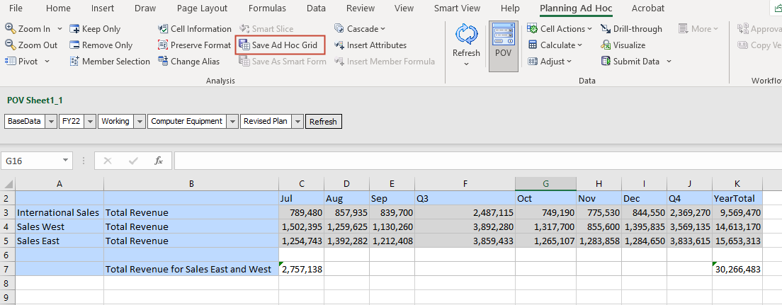
Saving the Ad Hoc Grid

In this section, you save the ad hoc grid.

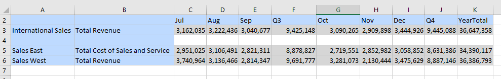
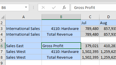
Update the ad hoc grid member selections to display the following example:
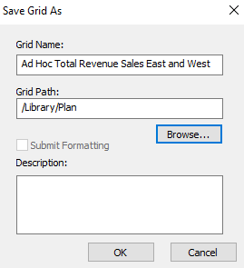
On the Planning Ad Hoc ribbon, click Save Ad Hoc Grid.
In Save Grid As, enter a grid name and select a grid path, and then click OK.
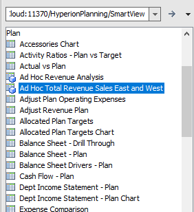
In the Smart View panel, locate the saved grid.
In the Smart View Panel, disconnect all connections and close Excel.

Setting the Smart View Ad Hoc Behavior

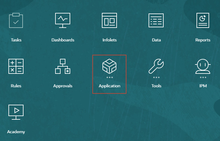
Access the Planning Vision sample application on the web.
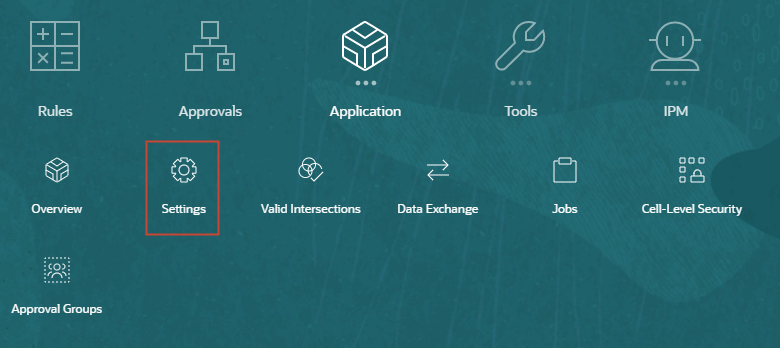
On the home page, click Application.
Click Settings.
In Application Settings, locate Smart View Ad Hoc Behavior and set it to Native.
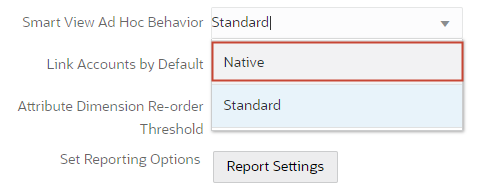
Click Save.
In the information dialog, click OK.
Log off Planning.
Launch Excel and reconnect to the Planning Vision application in your EPM Cloud instance.

Inserting Calculating and Non-Calculating Rows and Columns

You can insert calculating and non-calculating columns and rows within or outside the grid.

Inserted rows and columns, which may contain formulas, text, or Excel comments, are retained when you refresh or zoom in.

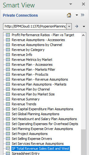
In the Smart View panel, locate the ad hoc grid you saved Ad hoc analysis mode.
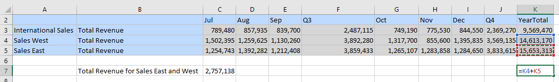
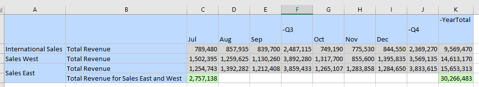
In an empty cell below the July column, enter a formula that adds the Total Revenue data for Sales East and Sales West. Here's an example:
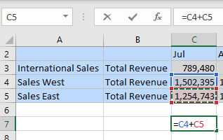
In cell to its left, enter the following comment: Total Revenue for Sales East and West .
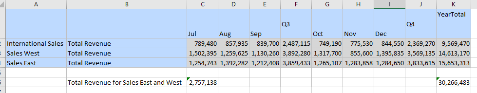
In an empty cell below YearTotal, enter a formula that adds the Total Revenue data for Sales East and Sales West - YearTotal.
On the Planning Ad Hoc ribbon, click Refresh.
The grid is updated.

Saving Ad Hoc Grids as Smart Forms

You can save your ad hoc grid, including the calculations and comments you added, as a Smart Form. Smart Forms support grid labels, along with business calculations in the form os Excel formulas and functions.

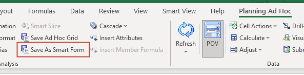
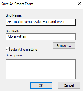
On the Planning Ad Hoc ribbon, click Save As Smart Form.
In Save As Smart Form, enter a grid name, select the grid path, select Submit Formatting, and click OK.

Tip:
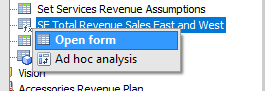
Selecting Submit Formatting saves any custom Excel formatting changes that have been applied to the grid.
Locate the Smart Form you save.
Right-click the Smart Form and select Open form.

The Smart Form is displayed.

Learn More

Related videos and documentation

Title and Copyright Information

Analyzing Plan Data in Smart View

F56075-01

April 2022

Analyzing Plan Data in Smart View

This software and related documentation are provided under a license agreement containing restrictions on use and disclosure and are protected by intellectual property laws. Except as expressly permitted in your license agreement or allowed by law, you may not use, copy, reproduce, translate, broadcast, modify, license, transmit, distribute, exhibit, perform, publish, or display any part, in any form, or by any means. Reverse engineering, disassembly, or decompilation of this software, unless required by law for interoperability, is prohibited.

If this is software or related documentation that is delivered to the U.S. Government or anyone licensing it on behalf of the U.S. Government, then the following notice is applicable:

U.S. GOVERNMENT END USERS: Oracle programs (including any operating system, integrated software, any programs embedded, installed or activated on delivered hardware, and modifications of such programs) and Oracle computer documentation or other Oracle data delivered to or accessed by U.S. Government end users are "commercial computer software" or "commercial computer software documentation" pursuant to the applicable Federal Acquisition Regulation and agency-specific supplemental regulations. As such, the use, reproduction, duplication, release, display, disclosure, modification, preparation of derivative works, and/or adaptation of i) Oracle programs (including any operating system, integrated software, any programs embedded, installed or activated on delivered hardware, and modifications of such programs), ii) Oracle computer documentation and/or iii) other Oracle data, is subject to the rights and limitations specified in the license contained in the applicable contract. The terms governing the U.S. Government's use of Oracle cloud services are defined by the applicable contract for such services. No other rights are granted to the U.S. Government.

This software or hardware is developed for general use in a variety of information management applications. It is not developed or intended for use in any inherently dangerous applications, including applications that may create a risk of personal injury. If you use this software or hardware in dangerous applications, then you shall be responsible to take all appropriate fail-safe, backup, redundancy, and other measures to ensure its safe use. Oracle Corporation and its affiliates disclaim any liability for any damages caused by use of this software or hardware in dangerous applications.

Oracle and Java are registered trademarks of Oracle and/or its affiliates. Other names may be trademarks of their respective owners.

Intel and Intel Inside are trademarks or registered trademarks of Intel Corporation. All SPARC trademarks are used under license and are trademarks or registered trademarks of SPARC International, Inc. AMD, Epyc, and the AMD logo are trademarks or registered trademarks of Advanced Micro Devices. UNIX is a registered trademark of The Open Group.

This software or hardware and documentation may provide access to or information about content, products, and services from third parties. Oracle Corporation and its affiliates are not responsible for and expressly disclaim all warranties of any kind with respect to third-party content, products, and services unless otherwise set forth in an applicable agreement between you and Oracle. Oracle Corporation and its affiliates will not be responsible for any loss, costs, or damages incurred due to your access to or use of third-party content, products, or services, except as set forth in an applicable agreement between you and Oracle.