3.3.4 Evaluate

Evaluate your model by reviewing diagnostic metrics and performing quality checks.

In some cases, querying dictionary views and model detail views may be sufficient to assess model performance. However, for a more thorough evaluation, you can compute test metrics such as Conditional Log-Likelihood, Average Mean Squared Error (AMSE), Akaike Information Criterion (AIC), and others.

Model Settings Information

Evaluate the model by examining the various statistics generated after model creation. These statistics provide insights into the model's quality.

%r
 
summary(MOD)

This script outputs a summary of a created exponential smoothing model, trained in the Oracle Database using the SALES_TIME_AMOUNT data. The summary confirms model type, input variables, target, forecast settings, and Oracle model metadata — all stored in the object MOD and available in the database as ESM_SALES_FORECAST_1.

Forecast

In this step, you will forecast sales for the next four quarters.

1. Forecast AMOUNT SOLD

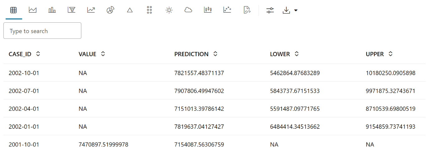
   The model ESM_MOD predicts four future values of AMOUNT_SOLD, along with lower and upper confidence bounds. The results are sorted in descending time order, displaying the most recent forecasted points first.

   %r
    
   modelDetails <- summary(MOD)
    
   PRED <- modelDetails$predictions
     
   z.show(ore.sort(PRED, by='CASE_ID', reverse=TRUE))

   
   
   
   
   

   The output is a table showing the forecasted values of AMOUNT_SOLD for the next 4 future CASE_ID periods (For example: quarters), sorted in descending order of time. This helps you view the most recent predictions at the top, providing a clear snapshot of expected future sales.

   Explanation of each column in the output:

   • CASE_ID:

     A unique identifier for each input record (or row) used during prediction. Helps track which prediction corresponds to which original data row.

   • Value:

     The actual (observed) value from the dataset, typically the true target/output variable.

   • Prediction:

     The predicted value generated by the model for that record. This can be a class label (for classification) or a numeric value (for regression).

   • Lower:

     The lower bound of the confidence or prediction interval. Indicates the lowest expected value with a given level of confidence (e.g., 95%).

   • Upper:

     The upper bound of the confidence or prediction interval. Indicates the highest expected value with a given level of confidence.

2. Chart Forecasted AMOUNT_SOLD Values with Confidence Intervals

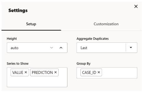
   To visualize the forecasted values in OML Notebooks, run the same query as above with the following chart settings:

   z.show(ESM_MOD.prediction.sort_values(by='TIME_SEQ'))

   
   
   
   
   
   
   
   
   

The line chart effectively illustrates how the model’s predictions track the actual observed values (Value) over time (time_id).

This completes the prediction step. The model has successfully forecasted sales for the next four quarters. These forecasts help track sales trends and provide valuable insights for inventory planning.