7.16 Orthogonal Partitioning Cluster
The ore.odmOC function builds an in-database model using the Orthogonal Partitioning Cluster (O-Cluster) algorithm.
The O-Cluster algorithm builds a hierarchical grid-based clustering model, that is, it creates axis-parallel (orthogonal) partitions in the input attribute space. The algorithm operates recursively. The resulting hierarchical structure represents an irregular grid that tessellates the attribute space into clusters. The resulting clusters define dense areas in the attribute space.
The clusters are described by intervals along the attribute axes and the corresponding centroids and histograms. The sensitivity argument defines a baseline density level. Only areas that have a peak density above this baseline level can be identified as clusters.
The k-Means algorithm tessellates the space even when natural clusters may not exist. For example, if there is a region of uniform density, k-Means tessellates it into n clusters (where n is specified by the user). O-Cluster separates areas of high density by placing cutting planes through areas of low density. O-Cluster needs multi-modal histograms (peaks and valleys). If an area has projections with uniform or monotonically changing density, O-Cluster does not partition it.
The clusters discovered by O-Cluster are used to generate a Bayesian probability model that is then used during scoring by the predict function for assigning data points to clusters. The generated probability model is a mixture model where the mixture components are represented by a product of independent normal distributions for numeric attributes and multinomial distributions for categorical attributes.
If you choose to prepare the data for an O-Cluster model, keep the following points in mind:
-
The O-Cluster algorithm does not necessarily use all the input data when it builds a model. It reads the data in batches (the default batch size is 50000). It only reads another batch if it believes, based on statistical tests, that there may still exist clusters that it has not yet uncovered.
-
Because O-Cluster may stop the model build before it reads all of the data, it is highly recommended that the data be randomized.
-
Binary attributes should be declared as categorical. O-Cluster maps categorical data to numeric values.
-
The use of OML4SQL equi-width binning transformation with automated estimation of the required number of bins is highly recommended.
-
The presence of outliers can significantly impact clustering algorithms. Use a clipping transformation before binning or normalizing. Outliers with equi-width binning can prevent O-Cluster from detecting clusters. As a result, the whole population appears to fall within a single cluster.
The specification of the formula argument has the form ~ terms where terms are the column names to include in the model. Multiple terms items are specified using + between column names. Use ~ . if all columns in data should be used for model building. To exclude columns, use - before each column name to exclude.
For information on the ore.odmOC function arguments, call help(ore.odmOC).
Settings for an Orthogonal Partitioning Cluster Models
The following table lists settings that apply to Orthogonal Partitioning Cluster models.
Table 7-18 Orthogonal Partitioning Cluster Model Settings
| Setting Name | Setting Value | Description |
|---|---|---|
|
|
|
A fraction that specifies the peak density required for separating a new cluster. The fraction is related to the global uniform density. Default is |
Example 7-19 Using the ore.odmOC Function
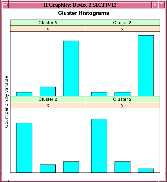
This example creates an O-Cluster model on a synthetic data set. The figure following the example shows the histogram of the resulting clusters.
x <- rbind(matrix(rnorm(100, mean = 4, sd = 0.3), ncol = 2),
           matrix(rnorm(100, mean = 2, sd = 0.3), ncol = 2))
colnames(x) <- c("x", "y")
x_of <- ore.push (data.frame(ID=1:100,x))
rownames(x_of) <- x_of$ID
oc.mod <- ore.odmOC(~., x_of, num.centers=2)
summary(oc.mod)
histogram(oc.mod)
predict(oc.mod, x_of, type=c("class","raw"), supplemental.cols=c("x","y"))
Listing for This Example
R> x <- rbind(matrix(rnorm(100, mean = 4, sd = 0.3), ncol = 2),
+             matrix(rnorm(100, mean = 2, sd = 0.3), ncol = 2))
R> colnames(x) <- c("x", "y")
R> x_of <- ore.push (data.frame(ID=1:100,x))
R> rownames(x_of) <- x_of$ID
R> oc.mod <- ore.odmOC(~., x_of, num.centers=2)
R> summary(oc.mod)

Call:
ore.odmOC(formula = ~., data = x_of, num.centers = 2)

Settings:
                  value
clus.num.clusters     2
max.buffer        50000
sensitivity         0.5
prep.auto            on

Clusters:
  CLUSTER_ID ROW_CNT PARENT_CLUSTER_ID TREE_LEVEL DISPERSION IS_LEAF
1          1     100                NA          1         NA   FALSE
2          2      56                 1          2         NA    TRUE
3          3      43                 1          2         NA    TRUE

Centers:
   MEAN.x   MEAN.y
2 1.85444 1.941195
3 4.04511 4.111740
R> histogram(oc.mod)
R> predict(oc.mod, x_of, type=c("class","raw"), supplemental.cols=c("x","y"))
             '2'          '3'        x        y CLUSTER_ID
1   3.616386e-08 9.999999e-01 3.825303 3.935346          3
2   3.253662e-01 6.746338e-01 3.454143 4.193395          3
3   3.616386e-08 9.999999e-01 4.049120 4.172898          3
# ... Intervening rows not shown.
98  1.000000e+00 1.275712e-12 2.011463 1.991468          2
99  1.000000e+00 1.275712e-12 1.727580 1.898839          2
100 1.000000e+00 1.275712e-12 2.092737 2.212688          2
Figure 7-4 Output of the histogram Function for the ore.odmOC Model

Description of "Figure 7-4 Output of the histogram Function for the ore.odmOC Model"