Example Using SqlGraphVisualization and PgxGraphVisualization
You can visualize SQL property graph queries using the oraclegraph Jupyter widget for interactive graph visualization. Additionally, you can load the graph into the graph server (PGX), run PGQL queries, and visualize the graph.
The following steps show you how to visualize and interact with your SQL property graphs in a Jupyter environment (either Jupyter Notebook or JupyterLab) using the graph visualization extension. The instructions assume that you already have a SQL property graph created in your Oracle AI Database 26ai. The example is based on the sample bank graph data (see Using Sample Graph Data) provided with the graph server installation in the database tables.
-
Open a new notebook and establish a connection to Oracle AI Database 26ai using the Python
oracledbdriver.import oracledb connection = connection=oracledb.connect( user=graphuser, password="<password_for_graph_user>", dsn="<hostname:port/dbservice>", print("Connection established successfully.") -
Run a SQL graph query on your property graph and visualize the query results using the graph visualization extension.
For instance, the following example runs a SQL graph query on
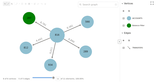
BANK_GRAPHand generates a visualization of the query results using theoraclegraphextension.from oraclegraph import GraphVisualization, SqlGraphVisualization # Define the query to fetch graph data query=''' SELECT * FROM GRAPH_TABLE (bank_graph MATCH (a WHERE a.ID=816) -[e]-> (b) COLUMNS (vertex_id(a) AS id_a, edge_id(e) AS id_e, vertex_id(b) AS id_b ) ) ''' # Initialize SqlGraphVisualization with the connection vq = SqlGraphVisualization(connection) # Execute the query graph_query = vq.visual_query(query) defaults_feature = { "interactionActive": True, "1stickyActive": True } base_styles = { "vertex": { "label": "${properties.ID}", "size": 20 }, "edge": { "label": "${properties.AMOUNT}" } } rule_based_styles = [{ "stylingEnabled": True, "component": "vertex", "target": "vertex", "conditions": { "conditions": [{ "property": "BALANCE", "operator": "<=", "value": 5000 }], }, "style": { "color": "green" }, "legendTitle": "Balance Filter", "legendDisplayed": True } ] settings = { "numberOfHops": 2, "showLegend": True, "defaults": defaults_feature, "baseStyles": base_styles, "ruleBasedStyles": rule_based_styles } # Create and display the graph widget bank_graph = GraphVisualization(data = graph_query, settings = settings) bank_graph.height = 600 display(bank_graph)The preceding code produces the following visualization result:
Figure: SQL Property Graph Query Visualization
-
Load the graph into the graph server (PGX) and run graph analytics.
The following example loads the graph into the graph server (PGX) and runs the Pagerank algorithm on the graph.
from oraclegraph import PgxGraphVisualization
from pypgx import setloglevel
from opg4py import graph_server

setloglevel("ROOT", "WARN")

base_url = "https://localhost:7007"
username = "graphuser"
password = "<password_for_graphuser>"

# Connect to graph server and create a session
instance = graph_server.get_instance(base_url, username, password)
session = instance.create_session("jupyter_session")

loaded_graph = session.read_graph_by_name("BANK_GRAPH", "pg_sql")

analyst = session.create_analyst()
pagerank = analyst.pagerank(loaded_graph, rank = "pagerank")
result_set = loaded_graph.query_pgql("SELECT x, x.pagerank MATCH (x) ORDER BY x.pagerank DESC LIMIT 10")
result_set.print()
The preceding code produces the following output:
+-----------------------------------------------------------------------------------------+ | x | x.pagerank | +-----------------------------------------------------------------------------------------+ | PgxVertex[provider=BANK_ACCOUNTS,key=387,ID=BANK_ACCOUNTS(387)] | 0.007292323575404966 | | PgxVertex[provider=BANK_ACCOUNTS,key=406,ID=BANK_ACCOUNTS(406)] | 0.006730094462320363 | | PgxVertex[provider=BANK_ACCOUNTS,key=135,ID=BANK_ACCOUNTS(135)] | 0.0067205459831892545 | | PgxVertex[provider=BANK_ACCOUNTS,key=934,ID=BANK_ACCOUNTS(934)] | 0.0066348438503635795 | | PgxVertex[provider=BANK_ACCOUNTS,key=397,ID=BANK_ACCOUNTS(397)] | 0.005693569761570974 | | PgxVertex[provider=BANK_ACCOUNTS,key=559,ID=BANK_ACCOUNTS(559)] | 0.005258438311460985 | | PgxVertex[provider=BANK_ACCOUNTS,key=352,ID=BANK_ACCOUNTS(352)] | 0.005216329599236731 | | PgxVertex[provider=BANK_ACCOUNTS,key=330,ID=BANK_ACCOUNTS(330)] | 0.005093350408942337 | | PgxVertex[provider=BANK_ACCOUNTS,key=222,ID=BANK_ACCOUNTS(222)] | 0.004682551613749817 | | PgxVertex[provider=BANK_ACCOUNTS,key=4,ID=BANK_ACCOUNTS(4)] | 0.004569682370461632 | +----------------------------------------------------------------------------------------- -
Run a PGQL query on the graph in the graph server (PGX) and visualize the query results using the graph visualization extension.
props={'size': 40}
# Initialize PgxGraphVisualization with the session
vq = PgxGraphVisualization(session=session)

base_styles = {
  "vertex": {
    "label": "${properties.ID}",
    "size": 10
  },
  "edge": {
    "label": "${properties.AMOUNT}"
  }
}

settings = {
    "showLegend": True,
    "baseStyles": base_styles,
}

query = '''
SELECT * FROM MATCH (v1)-[e]->(v2) ON {graph_name} LIMIT 100

'''.format(graph_name=loaded_graph.name)

# Fetch graph data as JSON
json = vq.visualize_query(query)

# Create and display the graph widget
graph = GraphVisualization(data=json, settings=settings)
graph.height = 800
display(graph)
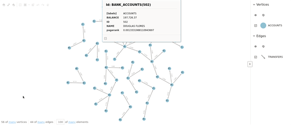
The preceding code produces the following visualization result:
Figure: Graph Visualization in the Graph Server (PGX)