Using the Jupyter Notebook Interface for PGQL Property Graphs
You can use the Jupyter notebook interface to create, load, and query PGQL property graphs through Python.
In addition, you can visualize PGQL property graphs using the graph visualization extension in both Jupyter Notebook and JupyterLab. See Getting Started with the Graph Visualization Extension in Jupyter Environments for more information.
The following steps show you how to create and visualize PGQL property graphs in a Jupyter environment (either Jupyter Notebook or JupyterLab).
-
Install the desired Jupyter Notebook interface (either Jupyter Notebook or JupyterLab).
-
Ensure that your Jupyter installation is added to the
PATHenvironment variable. -
Install the graph visualization extension in your Jupyter environment. See Installing the Graph Visualization Extension for Jupyter for more information.
-
Create a PGQL property graph using the OPG4Py Python API in a Jupyter notebook.
-
Establish a connection to the database using the Python
oracledbdriver.The following code shows how to connect to your local database:
import oracledb
host = "<host>"
port = 1521
service_name = "<service_name>"
dsn = f"{host}:{port}/{service_name}"

conn = oracledb.connect(
    user="graphuser",
    password="<password_for_graphuser>",
    dsn=dsn
)
jdbc_url = f"jdbc:oracle:thin:@//{host}:{port}/{service_name}"
print("Connection established successfully.")
To connect to an Autonomous AI Database, download the database wallet and unzip it to a secure directory on the machine running your Jupyter notebook. Then, connect using a
tns_aliasfromtnsnames.ora, as shown in the following code:import oracledb username = "adbgraphuser" password = "<password_for_adbgraphuser>" wallet_location = "<path_to_wallet_file>" wallet_password = "<password_for_wallet>" adb_tns_alias = "<tns_alias_in_tnsnames.ora>" connection = oracledb.connect( user=username, password=password, dsn=adb_tns_alias, config_dir=wallet_location, wallet_location=wallet_location, wallet_password=wallet_password, ) jdbc_url = f"jdbc:oracle:thin:@{adb_tns_alias}?TNS_ADMIN={wallet_location}" print("Connection established successfully.") -
Create a PGQL property graph using the
jdbc_urlcreated in the previous step.import opg4py pgql_connection = opg4py.pgql.get_connection("<username>", "<password>", jdbc_url) pgql_statement = pgql_connection.create_statement() create_pgql_graph = ''' CREATE PROPERTY GRAPH BANK_GRAPH_PGQL VERTEX TABLES ( BANK_ACCOUNTS KEY (ID) PROPERTIES (ID, Name, Balance) ) EDGE TABLES ( BANK_TRANSFERS KEY (TXN_ID) SOURCE KEY (src_acct_id) REFERENCES BANK_ACCOUNTS(ID) DESTINATION KEY (dst_acct_id) REFERENCES BANK_ACCOUNTS(ID) PROPERTIES (src_acct_id, dst_acct_id, amount) ) OPTIONS ( PG_PGQL ) ''' pgql_result_set = pgql_statement.execute(create_pgql_graph) pgql_statement.close() pgql_connection.close()
-
-
Run a PGQL query on the property graph and visualize the query results using
PgqlGraphVisualizationinoraclegraphJupyter extension.You can create a
PgqlGraphVisualizationinstance as shown in the following code examples:For Local Database
vq = PgqlGraphVisualization(
    "<db_username>",
    "<db_password>",
    connection={"dsn": f"{<host>}:{<port>}/{<service_name>}"},
)
For Autonomous AI Database (Wallet/tnsnames.ora)
vq = PgqlGraphVisualization(
    "<db_username>",
    "<db_password>",
    connection={
        "tns_alias": "<tns_alias_in_tnsnames.ora>",
        "wallet_location": "<wallet_location>",
    },
)
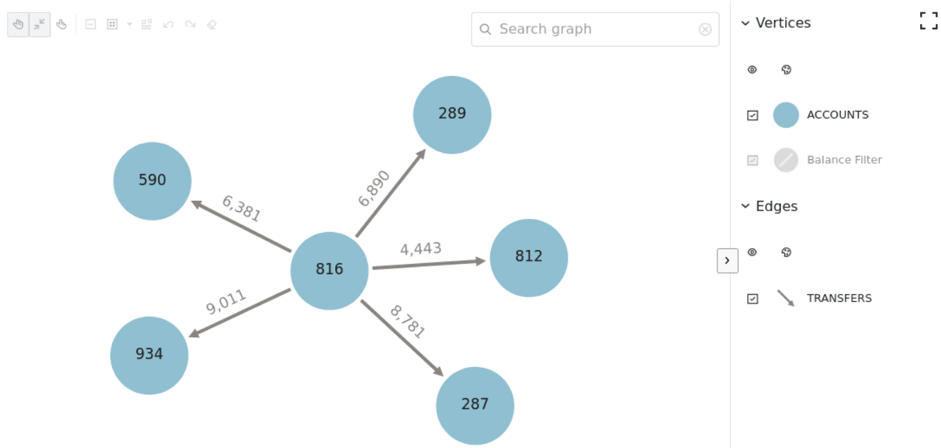
The following example shows how to visualize a PGQL query using
PgqlGraphVisualizationagainst the property graph created in step-4.from pypgx import setloglevel from oraclegraph import GraphVisualization, PgqlGraphVisualization setloglevel('ROOT', 'WARN') vq = PgqlGraphVisualization( "graphuser", "<password_for_graphuser>", connection={"dsn": f"<host_name:port>/<service_name>"}, ) query=''' SELECT * FROM GRAPH_TABLE (bank_graph_pgql MATCH (a) -[e]-> (b) WHERE a.ID=816 COLUMNS (a.ID AS src_ac, e.AMOUNT AS amount, b.ID AS dest_ac) ) ''' defaults_feature = { "interactionActive": True, "1stickyActive": True } base_styles = { "vertex": { "label": "${properties.ID}", "size": 20 }, "edge": { "label": "${properties.AMOUNT}" } } rule_based_styles = [{ "stylingEnabled": True, "component": "vertex", "target": "vertex", "conditions": { "conditions": [{ "property": "ID", "operator": "<", "value": 300 }], }, "style": { "color": "green" }, "legendTitle": "Balance Filter", "legendDisplayed": True } ] settings = { "numberOfHops": 2, "showLegend": True, "defaults": defaults_feature, "baseStyles": base_styles, "ruleBasedStyles": rule_based_styles } bank_graph = vq.visualize_query(query) bank_graph.height = 600 bank_graph.settings = settings display(bank_graph)The preceding code produces the following visualization result:
Figure: PGQl Property Graph Visualization
-
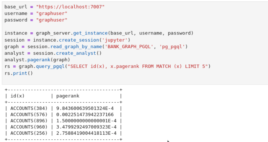
Load and analyze the property graph in the graph server (PGX).
The following example shows loading the PGQL property graph into the graph server (PGX) and running graph algorithms for analysis:
base_url = "https://localhost:7007"
username = "graphuser"
password = "<password_for_graphuser>"

instance = graph_server.get_instance(base_url, username, password)
session = instance.create_session('jupyter')
graph = session.read_graph_by_name('BANK_GRAPH_PGQL', 'pg_pgql')
analyst = session.create_analyst()
analyst.pagerank(graph)
rs = graph.query_pgql("SELECT id(x), x.pagerank FROM MATCH (x) LIMIT 5")
rs.print()
Figure: Running Graph Algorithms in Jupyter Notebook