Dynamic aggregation supports two “levels” of aggregation. Aggregating source data, from measuring components, items, or billed quantities is referred to as “Foundation” aggregation. Aggregation of aggregated data is known as “Composite” aggregation. Composite aggregation provides the ability to aggregate data from a set of other aggregations.

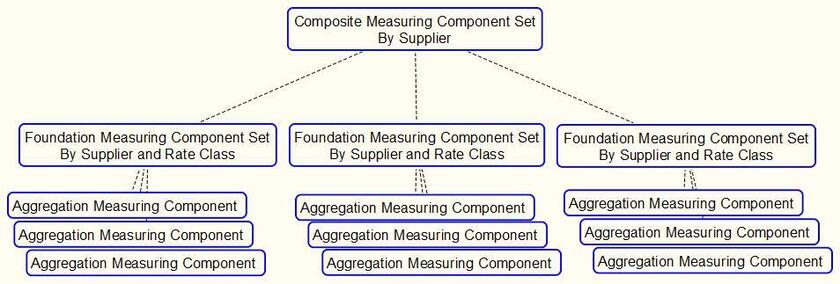
The diagram below illustrates a simple example of the relationship between foundation and composite measuring component sets. Each of the three foundation measuring component sets has a number of aggregation measuring component participants that aggregate data based on a set of dimensions and a particular supplier and rate class. Those in turn are participants in the composite measuring component set that aggregates based on the supplier (including data for all rate classes).

A common scenario where composite aggregation would be used is to consolidate data across several foundation aggregation measuring component sets that pulled data from a set of data sources ordered by precedence such that the best data was sourced when available and when not the aggregations fell back to a lesser quality data source:

In this example the goal of the first aggregation would be to retrieve as much interval data as possible where that interval data covered the entire period being settled for. The second aggregation would take scalar data for those instances where interval data was not available and apply a profile to produce the appropriate intervals. The third aggregation would fill in any remaining gaps that were not covered by interval or scalar data with estimations based various forecasting models.

At the completion of those first three aggregations there would be the full resolution of data for the customer base. However, the values would be spread out across many aggregation measuring components tied to those measuring component sets. This is where the composite aggregation functionality comes into play. The composite aggregation measuring component would reference the first three foundation aggregations and sum together the data from each aggregation into a single instance that represents the total usage for the period being settled.

Let’s look at a slightly more involved example. The diagram below illustrates a set of foundation aggregations based on:

This shows how the physical measuring component data (designated by Customer A, Customer B, etc.) will be aggregated into separate aggregation measuring components based on source of data (interval or scalar). Then it shows how those aggregations are then aggregated to produce a total number that represents all 3 aggregation sources merged together.