DMS Data Model Requirements and Configuration
This section describes the DMS Data Model process and data requirements. The data discussed in this section will be used by all DMS applications: Power Flow, Suggested Switching, Network Optimization, Feeder Load Management, Fault Location Analysis, and Fault Location Isolation and Service Restoration. It is intended to assist the customer during the DMS data modeling process. It is meant as an introduction, rather than a comprehensive reference.
Data Import and Build Process
The Oracle NMS shares a common model between the OMS and DMS applications. When a customer decides to implement DMS functionality they will need to layer engineering attributes (for example, impedances, voltage, ratings, and so on) onto the existing OMS connectivity model such that a power flow analysis can be conducted. The engineering attributes can be provided from GIS data, planning system data, protection coordination data, or a combination of multiple data sources. For data that is not readily available the Oracle Power Flow Engineering Data workbook can be used to supplement what may be missing.
The power flow runtime table configuration is created using the normal NMS model configuration practices and the data is populated during the normal build process. Initially the implementer needs to determine the availability of engineering attributes in the GIS and supplement what may be missing using flat files from an ancillary source (e.g., planning system) or provide the missing data in the Power Flow Engineering Data workbook. The DMS model configuration defines logic that determines from what source data should be obtained. For example the build process should first look in the GIS data for transformer kVA ratings, if this is determined to be null the process should next look in the Power Flow Engineering Data workbook tables for a device specific value, if this is determined to be null use a default defined in the workbook table. The logic is custom configured by the implementer for each attribute for each device type. The data requirements for each device type are discussed in the Modeling Device Data section below.
kVA Solutions
The data requirements for full power flow functionality are extensive and can take a significant amount of effort to validate before being cleared for use in production systems. A simpler data model that allows NMS to perform only kVA solutions (using nominal voltage) is also available.
kVA mode for solutions is configurable on a per-feeder basis through the Feeder Management tab of the Configuration Assistant. This allows the power flow engine to be rolled out into areas of the model as and when the data becomes available.
The following applications are supported using a kVA based solution: Power Flow, Suggested Switching, Feeder Load Management, and Fault Location Isolation and Service Restoration.
Note: Optimization and Fault Location Analysis will not function with a kVA based solution a full power flow model is needed for these two applications.
The following sections describe in detail the modeling and attribution required for all device classes for full power flow functionality. The reduced data set required for kVA solution is also discussed. Attributes that are not required for kVA solutions should be defaulted to reasonable values to enable consistency and validation checks to pass.
Modeling Device Data
This section will discuss each device type and the attributes required. The implementer will need to determine where this data can be obtained and think about the logic that will used in the model configuration for each attribute.
Sources
The customer must provide an equivalent source model for each source node defined in the data model. These source nodes represent constant voltage buses that are used to determine energization of the system and are generally located at feeder heads, the substation secondary bus generation sources, or the substation primary side bus. The required equivalent source parameters must represent an equivalent impedance looking up into the transmission system from the source node in question, in addition to voltage magnitude and angle. It is possible to model equivalent sources as zero impedance (i.e., 'infinite bus'), but this will impact the accuracy of short circuit calculations provided by the Power Flow solution. kVA modeling requirements for sources are: nominal voltage and initial angle.
Line Impedances
The customer must provide line data in one of three ways within the Power Flow Engineering Data workbook.
• The first and preferred way is to provide the phase impedance data for each three-phase line type. The phase impedance data must be the self and mutual impedance and shunt susceptance for each phase. The phase impedance data must be provided in the Line Phase Impedance tab of the power flow engineering data workbook. Oracle Utilities Network Management System Power Flow Extensions supports the modeling of symmetric and asymmetric lines. Lines are considered symmetric when the 3 phases have the same conductor type. Lines are considered asymmetric when the 3 phases have at least two different conductor types.
• The second way is to provide the sequence impedance data for each line. The sequence impedance table data must be the positive and zero sequence impedances and shunt susceptance for each line. The sequence impedance data must be provided in the Line Seq Impedance tab of the power flow engineering data workbook.
• The third way only applies to overhead lines and is used to provide the conductor and construction types for each line; this method cannot be used for underground cables. The power flow engineering data workbook uses Carson's Modified Equations to calculate phase impedance data from these inputs. This data must be provided in the Line Conductors tab and Line Constr Impedances tab of the power flow engineering data workbook. Line Conductors contains the individual conductor characteristics and limits associated to a conductor type. The Line Constr Impedance tab contains information regarding spacing and the types of conductor spacing combinations that occur in a particular customer data model.
For kVA solutions, all line impedance data can be defaulted to a generic conductor type. Line impedances are not used in the kVA engine.
Note: Line lengths will be automatically calculated by the NMS model build process and placed in the LENGTH column in the NETWORK_COMPONENTS table. If a project wishes to override this value, they can set up an override table (PF_LINES), which provides a mechanism to override the calculated value with a project defined value (for example, GIS attribute). If a value is populated in the PF_LINES table, the analysis will chose that value over the calculated value in the NETWORK_COMPONENTS table.
Transformers and Regulators
Oracle Utilities Network Management System Power Flow Extensions supports explicit modeling of multiple forms of power transformers, such as auto transformers, load-tap-changing transformers, step-up/step-down transformers and regulators. Each of these types of transformers and regulators require transformer characteristic data provided by the customer. The data should come from a combination of GIS data and/or PF Workbook data utilizing pf_xfmr_types and pf_ltc_xfmr tables. This data is written to pf_xfmr, pf_xfmr_tanks, and pf_xfmr_limits tables by the model preprocessor, which are read directly by Power Flow Service.
For voltage regulators, customers can model a single three phase device that represents three single phase devices in the field. This will allow independent regulation of voltage of each phase that mimics what occurs in the field. For this type of regulation, customers can set the regulator to unganged regulation and then provide a setpoint for each phase.
For kVA solutions, the data requirements for transformers and regulators are: Primary voltage, Secondary voltage, and rating.
NMS supports the ability model three winding transformers within the power flow data model. The modeling configuration needs to be setup in the preprocessing to break the device into three separate units within the NMS model. One to represent the load being served to the secondary side, one to represent the load being served to the tertiary side, and the third is needed to ensure the impedance model and fault calculations are accurate. Projects will generally only visualize the transformers serving load on the secondary and tertiary, the third should generally be hidden. The data for three winding units is provided in the Power Flow Engineering Data Workbook for a single device, upon extraction it will be split apart into three separate devices such that the data can then be mapped to the three devices within the NMS model. Projects have the ability to specify the step down voltages, ratings, tap configuration for both devices serving load to the primary and secondary. Please reference the following illustration as an example of how the device should modeled.
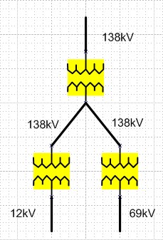
Note: The following configuration will be needed if transformers operate at a different voltage level than the system base. The primary and secondary ratios will need to be adjusted for the voltage the transformer outputs at the neutral tap position. The voltages configured for the unit should be based on what the voltages base that should be used for displaying results. For example, if a transformer had voltages levels from 138kV to 13.8kV on network at a 13.2kV system base. The primary ratio would be set to 1, the secondary ratio set to 1.04, the primary voltage would be set to 138kV, and the secondary voltage set to 13.2kV. If the device is auto regulating, the voltage target would then be set in P.U. based on a 13.2kV system base. With this scenario, the transferrer would output 13.8kV assuming no load and a 138kV input at the neutral LTC position. The power flow details would indicate this in the balloon as 1.04P.U. based on a 13.2kV system base.
Distributed Generation
Oracle Utilities Network Management System supports modeling of distributed energy resources for use in the power flow analysis. The runtime data for distributed energy resources is stored in table pf_dist_gen which is read directly by Power Flow Service. The parameters used within this table can be provided either via the customer’s data source(s), typically the GIS or via the Power Flow Workbook using table pf_dist_gen_data. The configuration supports small scale residential level generation all the way up to large spinning units that may be located at the substation. Generators must be configured with generation curves which represent the generator output for a particular condition. For example, a customer may configure three generation curves to categorize wind generation for Windy, Partly Windy, and No Wind. Using the Weather Zone Forecast Tool, a customer can set the gen schedule for the next 7 days, which drives what profiles are used for each type of generation.
For kVA solutions, the data requirements for Distributed Generation devices are: Rating and zone.
Capacitors and Reactors
Shunt (capacitor/reactor) parameters must be provided from the customer's data source(s), typically the GIS. These parameters are defined in the pf_capacitor_data table, which will be accessed by the Model Preprocessor, which in turn will write the pf_capacitors table, which will be read directly by the Power Flow Service.
Oracle supports the following types of shunt regulation:
• Voltage switched shunts: local or remote bus regulation
• Current switched shunts: local line or cable regulation
• kVAr switched shunts: local line or cable regulation
• Power-factor switched shunts: local line or cable regulation
• Temperature switched shunts: on and off temperature
• Time of day switched shunts: on and off time of day.
• Fixed shunts: no regulation
• Shunt sequence control
The supplied data for each shunt must indicate which type of regulation is to be used and the corresponding control attributes.
For kVA solutions, Capacitors and Reactors essentially need to be modeled in full.
Capacitors support two normal controls and one emergency control. Emergency control can overwrite those two controls. Two normal controls can have AND, OR logic.
Switch Ratings
Switch rating parameters must be provided from the customer’s data source(s), which is typically a GIS. These parameters are defined in the pf_switch_data table, and are accessed by the Model Preprocessor, which writes to the pf_switches_table, which is read by the Power Flow Service.
Predicting and reporting violations is a core advantage of the NMS distribution management system. Having accurate ratings and protection settings will allow the applications to generate meaningful violations. Data can be defaulted to reasonable values. Alternatively, they can be modeled as "Zero Impedance" devices to stop violation checking.
It should be noted that for protective devices that open to clear faults such as breakers, reclosers, and fuses the minimum pickup current should be used. For example, a breaker may be rated for 2000Amps, but the relay could be configured to trip at values greater than 600Amps; in this situation, a value of 600Amps should be configured for the devices normal, emergency short term, and emergency long term ratings.
For non-protective devices, the max continuous current rating of the device should be used which would represent the maximum amount of current the device could handle before failing. If desired, a separate emergency short term and long term limit could also be provided for non-protective devices. These values would represent a limit that could be sustained for a short duration of time (for example, 2-4 hours for short term and 24 hours for long term).
Within NMS, the capability exists to dynamically determine if protection reach issues exist on feeders. This occurs when the fault current on portions of a feeder are lower than the minimum pickup settings configured for the relay. In this situation, the fault current would not be seen as fault current and the device would not open to clear the fault. This can occur when feeders are switched abnormally and the length extended by picking up portions of adjacent feeders. To take advantage of this functionality, customers will need to configure the minimum pickup current for ground faults and for phase to phase faults for protective devices. For non-protective devices, or if this is not desired functionality, the values can be left null
Modeling Loads
Load modeling consists of basic load data which is used to determine average loading levels and load profile data, which is used to provide detailed information for load variation over time.
Basic Load Data
During modeling efforts, loads must be assigned to specific equipment types. The preferred approach is to insert a load (supply node) at the secondary of each underground and overhead distribution transformer. Supply nodes may also be created at primary metering points for cases where there is no voltage transformation or transformation is unknown or customer-owned.
For each load, a utilization factor can be specified, which represents the average loading level for the rated size of the transformer. For the most accurate power flow results, this data should be based on per-instance consumption data, which can often be obtained from historical billing information by dividing the total energy consumption of attached customers by the billing period and transformer rating.
The power flow data for load is defined using the table pf_load_data, which is read by the Model Preprocessor, which in turn writes the pf_loads table, which is read by the Power Flow Service.
Load Profile Data
Load profile data is used to model how load changes over time. A single load profile represents the change in load levels over a 24-hour period. Multiple profiles may be associated with a single load to represent different load behavior for different types of day (e.g., weekday, weekend) and for different temperatures (e.g., 80°F - 90°F, 90°F ‑ 100°F). The use of load profile data improves the accuracy of the DMS applications by providing more realistic loading scenarios for the current or predicted analysis time period. For example, profiles are used to verify switch plans, determine suggested switching recommendations, and generate daily and seasonal peak limit alarms.
The Oracle Utilities Network Management System supports a variety of sources of load profile data such as load class profiles or individual transformer profiles. Once processed, all profile data is placed in the pf_load_interval_data table. For load class profiles, the profile_id column in the pf_loads table can be set to point to the appropriate data in the pf_load_interval_data table. For transformer specific profiles, the adapter will populate a table pf_loads_profile_override; this table will be used to specify which transformers have specific profiles as opposed to just load class profiles. Anything defined in the pf_loads_profile_override table will override the profile_id field in the pf_loads table.
Load Class Profiles
Load class profiles represent typical load changes over time for a particular type or class of load, such as residential, commercial and industrial. This type of profile data can be obtained from general sources, or the customer can collect this data from typical customers or feeders. When using load class profiles, the load level at each load point is determined by combining the rated kVA with the load utilization factor and the class profile associated with that load. Load class profiles are useful where detailed data for each load is unavailable.
Transformer Profiles
Modern Meter Data Management (MDM) systems make it possible to collect detailed power usage histories for each customer. By aggregating individual meter loads to each service transformer, it is possible to create detailed load profiles for each transformer location. This data can be derived from either representative historical conditions or using predictive values, if the MDM system has this capability.
When using transformer profiles, all load data is derived from these profiles and basic load data such as the utilization factor is not used. The load profile input data can include both kW and kVAr values for load over the 24 hour period.
For kVA solutions, load modeling is still necessary. The amount of load modeling required will depend on the applications being used. If reasonably accurate future forecasting is required for Feeder Load Management, FLISR and/or Suggested Switching then detailed load profile curves will have to be generated. For real-time load flows only rating, utilization factor and power factor are required. Load will be scaled from SCADA data (where available).
Temperature Based Profiles
For all load profile sources, a temperature parameter can be used to add more granularity to the source data. Multiple profiles can exist that categorize how load behaves for a particular temperature range (for example, 80°F-90°F) for each day type. The power flow solution will use a zone based temperature forecast to determine what profile to use for each hour. For example, if it is forecast to be 60°F on a Monday at 9 a.m., the power flow solution would use the profile factor from the profile for a 60-70°F weekday morning at 9. For each day, multiple pieces of load profiles will be used to create a composite profile that represents the temperature profile for that day. Each load needs to be tied to an associated weather zone and the granularity at which temperature bands are defined will need to be defined in the pf_temperature_bands database table (for example, 10°F, 20°F, 5°F).
NMS provides a productized load profile adapter that assists with the creation of temperature based profiles. The adapter maintains a history of previously recorded load profile data and is continuously adjusting and updating profiles as new data is received. It adaptively learns what profiles look like for different day type and temperature combinations. The more data that is gathered by the adapter, the more accurate the profiles become. To use the adapter, you need to provide raw profile data aggregated to the transformer/primary meter level in a CSV file that matches the file format specified by Oracle (see the Oracle Utilities Network Management System Adapters Guide for more information). The adapter will determine what day type and temperature the profiles map to and then merge the data with existing data in the database. For example, if a new sample is received for Monday at 9 a.m. for profile "Sample_xfmr_1" at 65°F, the adapter needs to determine if the sample already exists; if it exists, the adapter calculates a rolling average based on the total number of samples received. Modeling Distributed Generation
Distributed Generation modeling consists of configuring parameters related to the unit that characterizes its power output. These parameters are defined in the pf_dist_gen_data table, which will be accessed by the Model Preprocessor, which in turn will create the pf_dist_gen table, which is read directly by Power Flow Service. If desired a utility can setup the model preprocessing such that all or only some of the attributes provided come from the GIS rather than the pf_dist_gen_data table. Distributed generation resources need be configured with the proper rating, impedance, power source (e.g., Wind, PV, Fossil Fuel, etc), and voltage regulation data that characterizes the unit. Each DER is also mapped to a set of profile data, which is used to provide detailed information regarding how a DER generates power over time. In certain situations such as a battery the profile will show when the unit is charging (consuming power) versus generating power.
Distributed Generation Profiles
Distributed Generation profile data is used to model how much power is contributed or even consumed over a period of time. Multiple profiles can be associated to a distributed generation resource to characterize how it behaves during different situations. For example a PV dist gen may have 6 different profiles to represent various levels of cloud cover (for example, Clear, Partly Cloudy, Cloudy, and so on). Each DER will also be associated to a particular power source to represent the type of distributed generation, for example Wind and PV may be project configured power sources. When forecast data is changed the power source attribute allows the Power Flow Service to determine what DERs need to have a profile change. For example if an admin changes the current days forecast from clear to cloudy you would only want to change the profiles for the PV dist gens but not the wind dist gens since that power source is unaffected as the wind speed is to remain the same. The use of distributed generation profiles improves the accuracy of the DMS applications by providing more realistic values of how distributed generation may actually be behaving in the field. For example PV output will be less during the early morning or late afternoon hours and nonexistent at night. During a cloudy day the output will be less than on a clear day. All of these situations can be handled with properly configured profiles.
Generation of PV Profiles
If desired a utility can use the product profile adapter to create PV profiles based for a predetermined set of day types (for example, Cloudy, Clear, Partly Cloudy, and so forth). When PV profile creation is configured the adapter will create PV profiles based on a set or specified configuration options. The PV profile creation will be based on a specified lat/long and time of year, this way each time the adapter is run a new set of accurate PV profile curves will be generated and loaded into the DB for use by power flow services. A command line option (-createPvOnly) when running the adapter will also exist to force the adapter to just generate the PV profiles and not load any load profiles into the DB.
Net Metered Profiles
If utilities are providing net metered profiles the Profile adapter can be configured to add back in the load served by the residential distributed generation resources such that a true load profile is provided to NMS for use within the power flow analysis. For example if you have a service transformer serving one customer and that customer consumes 100kW. If PV is present at that customer premise producing 40kW on a sunny day the power required from the utility to meet the load is 60kW. In this case the meter only telemeters 60kW even though the customer consumed 100kW. Since loads need to be split from distributed generation resources in the NMS network model we want the true load consumed by the customer not the net metered load. The adapter will be responsible for identifying dist gens below a service transformer and add the load served back into the net metered profile.
Catalog Tables
The catalog tables identified in this section must all be populated by the customer. The Power Flow Engineering Data Excel workbook should be used as a template to assist the customer in identifying source data locations (planning power flow data, database tables and so on), defining a data export mechanism, and specifying the Oracle table names, columns, and data formats into which the source data must be imported. See the example workbook in the Oracle Utilities Network Management System product directory location: $NMS_BASE/OPAL/workbooks.
DER and the Weather Zone Forecast
A utility has the ability to provide forecast data for various types of DER resources that are present within the electrical network. The NMS categorizes DERs into the following forecasts categories:
• Weather Affected DERs
• Utility Scale DERs
• Demand Response Groups
The following sections will describe how to configure them, and provide the required forecast data.
Weather Zones
A utility has the ability to configure different weather zones within the NMS data model such that different distributed generation profiles can be used within each of the different zones to characterize the real-time and forecasted generation output. For example, if the "coastal" zone is cloudy, a user could set the forecast for PV to use a cloudy profile in the coastal zone, but all other zones would use the clear profile. The weather zone configuration is also used by loads to adjust load profiles as temperature changes. DERs technology types (e.g., PV, Wind, etc.) that are mapped to weather zones should be weather affected DERs only. For example, a large utility scale diesel generator would not be mapped to a weather zone since its forecast and output is independent of weather conditions.
If a utility wishes to configure weather zone functionality, data needs to exist that maps each distributed generation and load resource in the NMS data model to one of the applicable zones. The preferable location for this data would be the GIS, but, if needed, the data could be placed in the customer specific Power Flow Engineering Data workbook. This data needs to be brought across during the model build into the ZONE columns of the PF_DIST_GEN and PF_LOADS tables. The value populated will need to map to a configured zone in the PF_WEATHER_ZONE table.
Once Weather Zones have been configured, the utility has the ability to provide a forecast for each zone that forecasts how the DER resources for each power source will behave for the current day plus the next six days. This forecast should also include a temperature forecast for each applicable zone; this will be used to adjust load profiles as temperature changes.
During implementation, a utility needs to determine how they would like to use the weather zone forecast functionality.
• They could have an administrator use the Weather Zone Forecast tool to set the generation profile daily for each zone and power source. The power flow solutions will then use the profiles that have been set for the day in the real-time solutions and forecasts.
• For more advanced forecasting, they could use an external interface (e.g., weather feed) to populate the PF_WEATHER_ZONE_FORECAST table for each hour of the day with what generation profile to use. This would allow for more granular refinement of the power flow solutions. In this scenario the utility would not use the Weather Zone Forecast tool to set the weather forecasts.
• Alternatively, they could provide direct scaling factors to use for each hour instead of what profile to use for each hour; the input method can be configured with the distGenDefault SRS rule.
Whichever method is used, the entire forecast for each zone must be provided with the same method (profiles or scaling factor) for each power source.
Temperature forecasts can be provided for US customers using a product adapter that interfaces to a weather data server. Alternatively, an implementer could build a custom adapter that would provide temperature forecasts on a zone basis from an alternate resource such as utility specific forecasts (see the Oracle Utilities Network Management System Adapters Guide for more information).
Large Scale Utility DERs
Large scale utility DERs are categorized as units that are large in scale and unaffected by weather. An example would be a diesel generator or large battery that has an output that is unaffected by weather. For these units, the forecast is provided for each individual unit and they are not aggregated together like DERs within weather zones. It may be entirely plausible to have two large batteries in close proximity to each other but their forecasts could be drastically different.
If a utility wishes to categorize a DER resource as being outside of a weather zone the ZONE field within the PF_DIST_GEN database table should be configured within the alias of the unit. The preferable location for this data would be the GIS, but if needed the data could be entered in the utility’s Power Flow Engineering Data workbook. This data will need to be brought across during the model build. A corresponding power source also needs to be configured for the unit (for example, Diesel, Gas, Battery, etc.)
Once the large scale DERs have been configured, the utility has the ability to provide a forecast for each unit that forecasts the output for the current day plus the next six days. It is expected that an external system would be used to populate the forecasts for these units and the data is stored in the PF_DER_FORECAST database table. Within this table a key corresponding to a distributed generation profile can be provided (for example, on, off, peak shave, and so forth). Alternatively, a utility could provide direct scaling factors to use for each hour instead of what profile to use for each hour, the input method can be configured with the distGenDefault SRS rule. With either method the entire forecast for all units must be provided with the same method (profiles or scaling factor) for each power source. The NMS has a DERMS adapter product that is capable of taking a CSV or RDBMS based forecast from an external system for use by the NMS (see the Oracle Utilities Network Management System Adapters Guide for more information).
Demand Response Groups
A utility has the ability to configure different demand response groups (DR groups) within the NMS data model such that different DR profiles can be used within each of the different groups to characterize the real-time and forecasted DR scenarios. For example, the ability to simulate a DR group dropping load for 2 hours during a peak load day.
If a utility wishes to configure demand response group functionality, data would need to exist that maps each DR resource in the NMS data model to one of the applicable demand response groups. The preferable location for this data would be the GIS, but, if needed, the data could be placed the utility’s Power Flow Engineering Data workbook. This data will need to be brought across during the model build into the ZONE column of the PF_DIST_GEN table. The value populated will need to map to a configured zone in the PF_DEMAND_RESPONSE_GROUPS table.
Once the demand response groups have been configured, the utility has the ability to provide a forecast for each demand response group that forecasts the output for the current day plus the next six days. It is expected that an external system would be used to populate the forecasts for these units and the data is stored with NMS DB table PF_DEMAND_RESPONSE_FORECAST. This table can have a key corresponding to a distributed generation profile (for example, on, off, etc.). Alternatively, a utility could provide direct scaling factors to use for each hour instead of what profile to use for each hour; the input method can be configured with the distGenDefault SRS rule. With either method, the entire forecast for all units must be provided with the same method (profiles or scaling factor) for each power source. The NMS has a DERMS adapter product that is capable of taking a CSV or RDBMS based forecast from an external system for use by the NMS (see the Oracle Utilities Network Management System Adapters Guide for more information).
DER and Weather Forecast Tables
PF_WEATHER_ZONE
Column | Comments |
|---|---|
ZONE_NAME | Name of the generation zone (e.g. Desert, Coastal, Mountain) |
DISPLAY | Boolean to indicate whether or not to display the zone on the user interface. If set to 'Y' display the zone if 'N' do not display the zone. This would be used by a utility that has many zones with some of them being fed by an automated weather feeder and others that are not. With this the utility could filter some of the zones out they don't need to display. |
EDITABLE | Boolean to indicate whether or not the zone is user editable using the user interface. If set to 'Y' allow a user to edit generation profiles for the zone from the user interface. If 'N' do not allow a user to edit the generation profiles for the zone, this would generally imply the zone is being set from an automated weather feed. This would be used by utilities that have many zones with some of them being fed by an automated weather feeder and others that are not. With this the utility could filter some of the zones out they don't need to edit. |
Latitude | The latitude of the center of the weather zone. |
Longitude | The longitude of the center of the weather zone. |
PF_WEATHER_ZONE_FORECAST
Column | Comments |
|---|---|
ZONE | Zone the forecast is applicable to. |
DATE_TIME | The date and time the forecast is applicable to. |
POWER_SOURCE_X (depends on the number of power sources configured such as wind, PV, etc.) | Key to the profile for the specified fuel type. Will be an integer value that represents a profile configured for the power source. Alternatively if the power source is configured for scale factors as the input this will be a float representing the scaling factor. |
TEMPERATURE | The temperature in either Fahrenheit or Celsius for the day, zone, and hour. This is used to adjust load profiles. |
PF_DEMAND_RESPONSE_GROUPS
Column | Comments |
|---|---|
DR_GROUP_NAME | The name of the demand response group. |
DISPLAY | Boolean to indicate whether or not to display the zone on the user interface. • Y: display the zone. • N: do not display the zone. |
MW_LOAD_DROP | The amount of load in MW that can be dropped with the group. |
PF_DEMAND_RESPONSE_FORECAST
Column | Comments |
|---|---|
DR_GROUP_NAME | Group the forecast is applicable to. |
TEMPERATURE | The temperature forecast for the demand response group. |
DATE_TIME | The date and time the forecast is applicable to. |
POWER_SOURCE_TYPE | Key to the demand response type. |
FORECAST_VALUE | Will be an integer value that represents a profile configured for the power source. Alternatively, if the power source is configured for scale factors as the input, this will be a float representing the scaling factor. |
PF_DER_FORECAST
Column | Comments |
|---|---|
RESOURCE_NAME | The name of the resource the forecast is applicable to. |
DATE_TIME | The date and time the forecast is applicable to. |
POWER_SOURCE_TYPE | Key to the generator power source type. |
FORECAST_VALUE | Will be an integer value that represents a profile configured for the power source. Alternatively, if the power source is configured for scale factors as the input, this will be a float representing the scaling factor. |
Seasonal and Temperature Limits
The power flow analysis can be configured to work with seasonal or temperature based limits when specifying ratings for power transformers and conductors. For these types of devices, the upper limit that the device can be pushed to is heavily dependent upon the ambient air temperature (in general, these devices can be pushed harder when the temperature is cooler since natural cooling can occur). Both the seasonal and temperature based approaches represent a mechanism to specify what the ambient air temperature is doing — with the temperature based approach providing much more possibility for granularity. Both approaches are global in nature so a project cannot specify one type of configuration for one area of the model but another approach for another area. Any ratings provided for switches will have the standard concept of normal, short term emergency, and long term emergency limits.
Configuration of Seasonal Limits
Seasonal Limits define a set of ratings that are applicable for predefined seasons. The power flow analysis will utilize the proper ratings based on the date of the power flow solution. For example, a project may configure two seasons (Winter and Summer); during the winter months, the defined winter ratings will be used for transformers and conductors, and for the summer months, the summer ratings will be used. Seasonal Limits can be enabled in the power flow analysis by following the steps below.
1. The USE_TEMP_LIMITS SRS rule should be configured with a value of no to enable seasonal limits within the analysis and also enable any user interface items that allow the user to specify the season.
2. The PF_SEASONS_DEF table needs to be configured and is used to store information related to season definitions used by power flow. The main points of configuration will be the season name and the start and end dates. The PF_SEASONS_DEF table should be defined in the [project]_pf_seasons.sql file.
PF_SEASONS_DEF
Column | Comments |
|---|---|
SEASON_NUMBER | The integer key corresponding to the season |
SEASON_NAME | The name of the season (for example, Summer, Winter) |
SEASON_START_DAY | The integer start day of the season |
SEASON_START_MONTH | The integer start month of the season |
SEASON_END_DAY | The integer end day of the season |
SEASON_END_MONTH | The integer end month of the season |
3. The integer value assigned to each season will need to correspond back to the same integer key assigned to transformer and conductor seasonal limits defined in the Power Flow Engineering Data workbook. The relevant transformer limits will be defined on the workbook's Power Xfmr Limits tab. The relevant conductor limits will be defined on the Line Phase Impedances, Line Seq Impedances, and/or Overhead Line Conductors tabs, depending on which method was used to provide the conductor impedances data. For each season, a set of limits will need to be provided for a normal, emergency short term, and emergency long term rating.
Configuration of Temperature Limits
Temperature Limits define a set of ratings that are applicable for predefined temperature bands. The power flow analysis will utilize the proper ratings based on the forecast temperature for the date and time of the power flow solution. So, for example, the configuration may be set up such that conductors and transformers will have a limit defined for each 20°F range of temperature. The limit used for each power flow solution will be based on the forecast temperature for the date and time the solution is for and weather zone the device is in. Therefore, while looking at forecast power flow solutions for a device, it may be possible to see the upper limit changing as the temperature changes throughout the day. This is the one big differentiator between seasonal based limits and temperature based limits; with the temperature based limits, the limit used has the possibility to change hour by hour as temperature changes whereas seasonal limit the same limit will be used for a larger date range. Temperature limits can be enabled in the power flow analysis by following the below steps.
1. The USE_TEMP_LIMITS SRS rule should be configured with a value of yes to enable temperature limits within the analysis and also enable any user interface items that allow the user to specify the temperature.
2. The PF_TEMPERATURE_BANDS table will need to be configured and is used to store information related to the number and range of each temperature band. The main points of this table will be setting an integer value that represents the band and the upper limit of the band; the lower limit will be based on whatever is configured as the upper limit from the previous band. The units on this table do not matter as long as the units when providing the data are all kept consistent; for example, when defining temperature bands, if the units could be in Fahrenheit or Celsius as long as the weather feed providing the forecast data is providing data with the same scale, the proper limit will be chosen.
Note: This table is shared configuration with defining of temperature bands for load profiles so the IS_LIMIT column needs to be set to "Y".
PF_TEMPERATURE_BANDS
Column | Comments |
|---|---|
TEMP_INDEX | The integer key corresponding to the temperature band |
UPPER_LIMIT | The upper limit of the temperature band |
IS_LIMIT | Specifies Y/N if this temperature band is for limits or profiles |
3. The integer value assigned to each temperature band will need to correspond back to the same integer key assigned to transformer and conductor temperature limits defined in the Power Flow Engineering Data workbook. The relevant transformer limits will be defined on the workbook's Power Xfmr Limits tab. The relevant conductor limits will be defined on the Line Phase Impedances, Line Seq Impedances, and/or Overhead Line Conductors tabs depending on which method was used to provide the conductor impedances data. For each season, a set of limits need to be provided for aa normal, emergency short term, and emergency long term rating.
4. A weather feed or custom integration will be needed to populate PF_WEATHER_ZONE table with temperature forecast information for each weather zone. This weather feed will be used by the power flow analysis to determine which limit to use for the real-time power flow solutions and forecast solutions; the forecast temperature will drive which of the predefined limits is used. For example, if a power flow solution being conducted at 9:30 a.m. has a forecast temperature of 65°F, the predefined rating for the 60°F-70°F band will be used.
Note: It is possible to configure a temperature measurement for SCADA telemetered power transformers. In this situation, the analysis will use the SCADA‑provided temperature rather than the forecasted temperature for the device's weather zone when choosing the limit in the real-time solution. For all forecast solutions, the weather feed temperature will still be used for choosing the limit.
5. Power transformers and conductors need to be mapped to a relevant weather zone such that the analysis can determine the applicable temperature to use for each device. The weather zone for transformers is mapped to the ZONE column in the PF_XFMRS table. The weather zone for lines is mapped to the ZONE column in the PF_LINES table.
Bellwether Meter Voltages
In real-time mode, Optimization is capable of making use of bellwether meter voltages. The voltages will be used as an input into the optimization algorithm to ensure that voltage violations are not created on the secondary network serving customer meters. By using voltage telemetry, the Oracle Utilities Network Management System can begin to learn the difference between the solved power flow voltage versus the actual telemetered voltage and make estimates as to what the secondary service drop may be between a service transformer and the bellwether meter location. If a customer strategically choses bellwether meter locations at points that experience the lowest voltage on a feeder, it will help ensure that the optimization does not create voltage issues in scenarios like Conservation Voltage Reduction (CVR) where the voltage is lowered to reduce demand. Oracle recommends that customers choose two to three metering points per regulation zone on a feeder. These voltages can come from field devices (for example, sectionalizers, reclosers, capacitors, and so forth) that are capable of telemetering voltage, but would be most useful at customer meters. For more information on configuration of the bellwether meter voltages, please see the SCADA Configuration for Bellwether Meters section in the Building the System Data Model chapter of the Oracle Utilities Network Management System Adapters Guide.
Viewing Power Flow Attributes
Power Flow attributes can be configured to display within the NMS Attribute Viewer. This would enable a DMS customer to see power flow attributes in addition to normal GIS attributes when using this tool. The Model Workbook is setup to programmatically determine relationships between the model tables and join the related tables together when generating attribute view. The tool tab Generate Attribute View with Supporting Tables check box enables this functionality.
To enable/disable the attributes that will display within the NMS attribute viewer, a project needs to populate a display name in the Display Name column of each applicable power flow tab within the model workbook (for example, pf_loads, pf_dist_gen, pf_xfmrs, and so forth).
It is recommended that projects use a key prefix in each of the display names so a user can easily see which attributes are GIS display‑only and which are power flow attributes that are used in the power flow analysis. For example, a project could use a prefix of "PF_" on each power flow related attribute.