24.1 Creating Non-Maturity Products Model

To create a new Non-Maturity Products Model Analysis Rule, perform the following steps:

1. Navigate to the Non-Maturity Products Model Analysis Summary Page.
2. Click Add . The Create Non-Maturity Products Model Analysis Page will be displayed.

   Figure 24-1 Creating Non-Maturity Products Model Analysis Rule

   
   

   

   
   
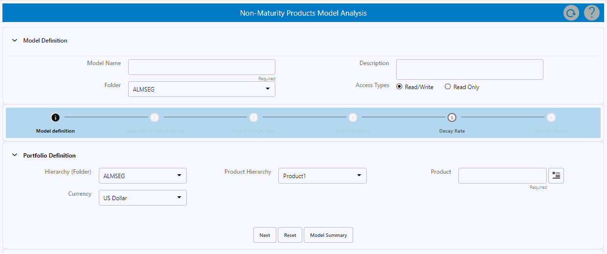
3. Enter the details shown in the following table.

   Table 24-2 List of process details used for Creating Non-Maturity Products Model Anal

   Fields	Description
   Model Name	Enter the name of the Non-Maturity Products Model Analysis Rule. This should be unique name. This field accepts Alpha Numeric value. Special characters are not allowed.
   Description	Enter the description of the Non-Maturity Products Model Analysis Rule. The maximum limit of this field is 300 characters. You can enter special characters in this field.
   Folder	Select the folder where you want to save the Non-Maturity Products Model Analysis Rule.
   Access Type	Select Access Type as Read-only or Read/Write.
   Hierarchy (Folder)	Select the folder where product is stored on which model need to be build.
   Product Hierarchy	Select the Product Hierarchy from available list of hierarchies in selected folder.
   Product	Based on the selected product hierarchy in model definition UI, Hierarchy Browser will expand the product hierarchy and you can select any parent/leaf node by clicking on the view button next to the product in the model definition screen.
   Currency	Select the currency for the Non-Maturity Products Model Analysis Rule. Only one currency can be selected for a particular model.

4. Click Apply to navigate to the Exploratory Data Analysis section.

   Figure 24-2 Creating Non-Maturity Products Model Analysis Rule - Exploratory Data Analysis section

   
   

   

   
   

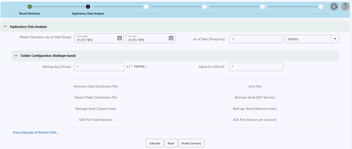
   The Exploratory Data Analysis Window will help you to perform EDA calculations and get a glimpse of data being used for modelling.

5. Enter the following details in the Exploratory Data Analysis window.

   Table 24-3 Fields on Exploratory Data Analysis

   Fields	Description
   Model Population (As of Date Range)	You can select a date range which will define the historical period within which data needs to be picked for Model creation By default, the Date range would be populated as below: End Date: Max (As of Date) available in Model input Table. Start Date: Max [min (As of Date), End Date – 10 Years]. Default values are populated from FSI_AUDIT_NM_LOAD_BATCH table.
   As of Date (Frequency)	The default value of this field is one month. As of Date (Frequency) defines on what regular intervals, data needs to be picked from the input table. For example, you can have historical period as last three years, in those three years at what regular interval data needs to be picked up from history table that would be defined by As of Date (Frequency).
   Moving average period for Bollinger Band	The default value of this field is one month. The Moving Average period defines the historical term over which the moving average needs to be calculated for Bollinger band formation.
   Sigma Co-efficient (Bollinger Band)	The default value of this field is 1. Sigma Co-efficient defines the outliers, any number which is (sigma coefficient * standard deviation) away from the mean, will not be considered for calculations. This field accepts Integer and Decimal values in the range 0 – 10.

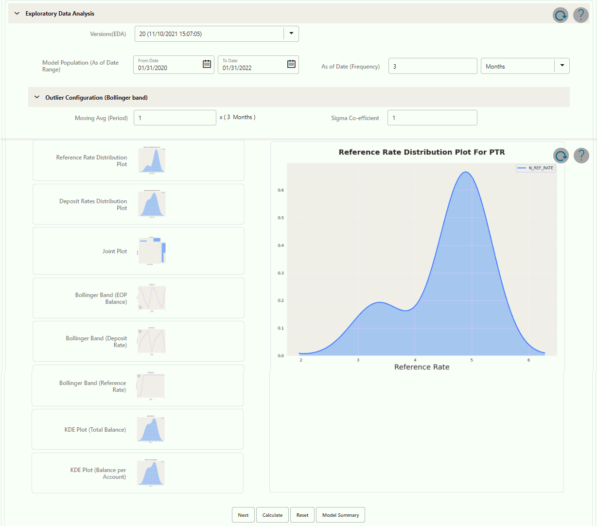
6. Click Calculate to perform Exploratory Data Analysis and get EDA plots. You can refresh the window using the Refresh button to check if the EDA is completed. When you open EDA window first time for a particular model, Version(EDA) field would not appear as there is no previous version to display. Subsequently, when first version is created and you go for second version, version (EDA) tab will start appearing with previous EDA versions. When EDA version is submitted, a message will appear with version number. You get a pop-up in case last run version was failed. If run was successful, latest version would appear on the UI, when you log back in. Reset button resets the entered values to their default values.

   Figure 24-3 Exploratory Data Analysis section

   
   

   

   
   
7. Click Next to navigate to the Pass-Through Rate Calculations window.

   Figure 24-4 Pass-Through Rate Calculations

   
   

   

   
   
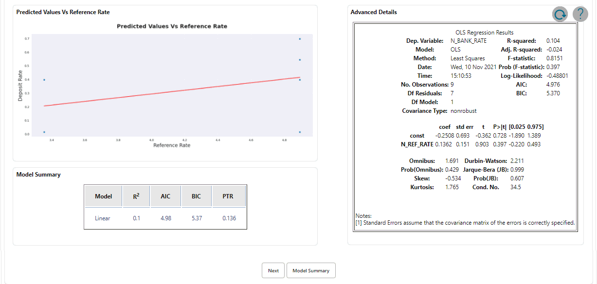
8. Click Calculate to view all the evaluation parameters and quality plots. Pass-Through Rate calculations are submitted, a message appears with version number. If you come back after some time, you get a pop-up in case last run version was failed. This window shows all the model quality parameters and graphs. At this stage, Pass through rate or beta between market rate and deposit rate is calculated. You can zoom the graph to enhance visibility. Following Advanced Details Window will help you to evaluate the model fit.

   Figure 24-5 Advanced Details

   
   

   

   
   
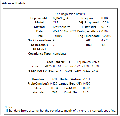   The Model parameters like R², AIC, BIC and regression co-efficient will be shown under model summary.(how much change in market rate is passed on to the deposit rate).

   Figure 24-6 Model Summary

   
   

   

   
   

   At any stage if user would like to come out of the model analysis module, one can Click on Model Summary button and go back to Non-Maturity products model summary screen and come out of modelling module.

9. Click Next to navigate to the Stable Balance Calculation section. This window shows the Projection period. You can set it as required. Projection period can be only be positive integers which will act as multiplier to As of Date (Freq). E.g. if as of date (Freq) is quarter and projection period is 8 * As of Date (Freq), it implies projection period is 2 years.

   Figure 24-7 Stable Balance Calculation

   
   

   

   
   
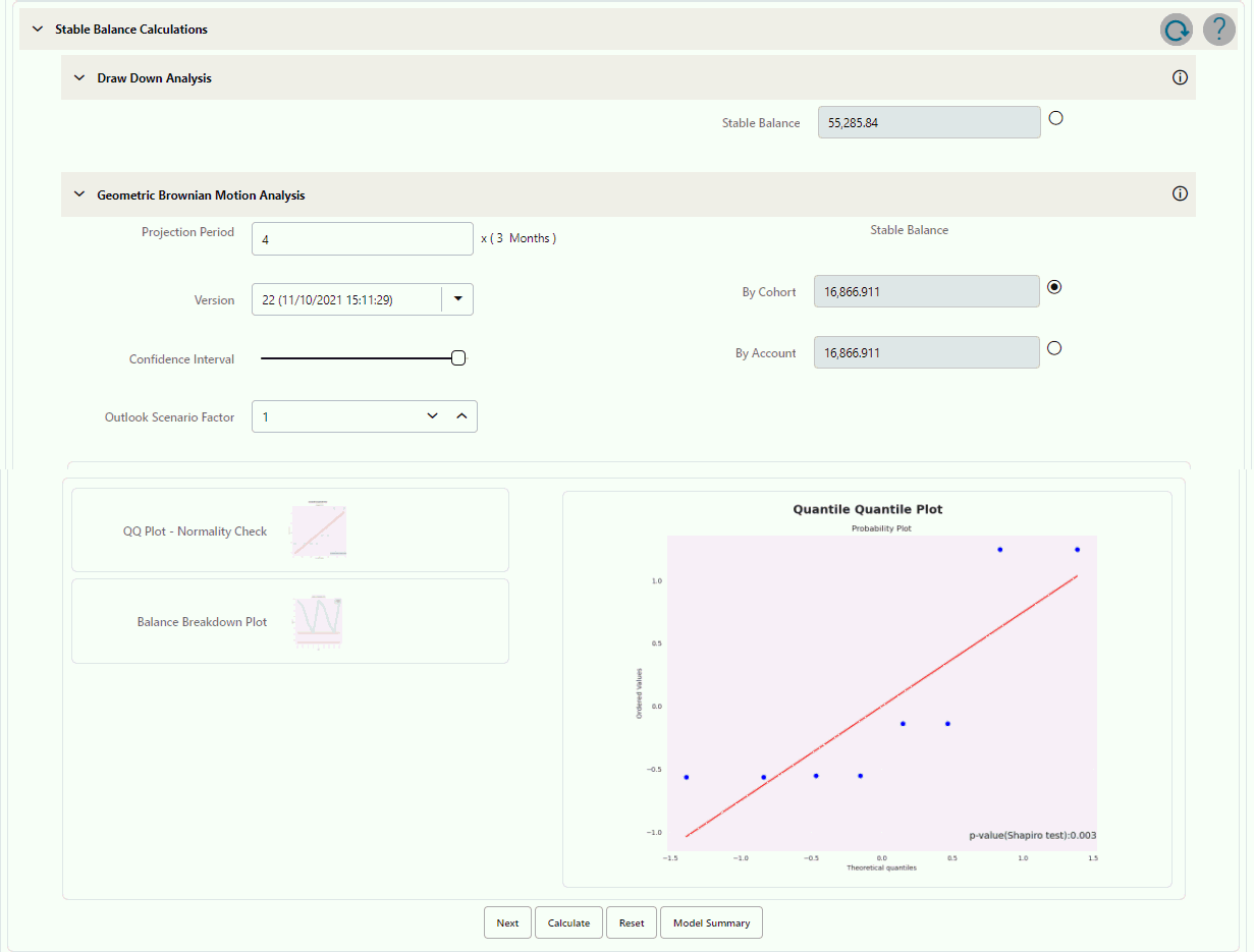
10. To calculate Stable Balance, you can use following methods:
    • Draw Down Analysis
    • Geometric Brownian Motion

    Draw Down Analysis: The Draw Down Analysis calculates each period’s Run-offs in the historical period and subtracts the maximum Run-off from the most recent total balance to arrive at stable balance.

    Geometric Brownian Motion: This approach will first calculate the past Run-offs volatility and assuming normal distribution of Run-offs, accept confidence interval as user input, projection period for time adjustment, and outlook scenario factor (volatility multiplier) as input from the user. After clicking calculate, the stable balance would be shown at cohort/account level using both cohort level and account level volatility and saved against version.

    The confidence interval slider field has a range of 0 – 100% and by default value as 95% and Outlook scenario factor (Volatility Multiplier) is set at 1 (Default Value).

    The range of outlook scenario factor is 0.01 to 1.99.

    You can change any of the inputs and generate multiple versions.

    A radio button is available for each method. Stable balance can be calculated with multiple methods, so before proceeding to next step, you must select one radio button to confirm one stable balance on which rest of the subsequent processing will take place. When this window is displayed first time, after pressing the Calculate, stable balance is calculated for both methods, Drawdown analysis and Geometric Brownian Motion. In subsequent runs, if any of projection period, confidence interval or Scenario factor is changed, then new version will be generated only for GBM. When you click Calculate button, then a pop up is displayed: " GBM version xyz is submitted’. If you come back and version is failed, a pop up is displayed: "‘GBM version xx is failed’ and UI will revert back to last successful version".

11. Click Next to navigate to the Decay Rate Calculations Section.

    Figure 24-8 Decay Rate Calculations

    
    

    

    
    
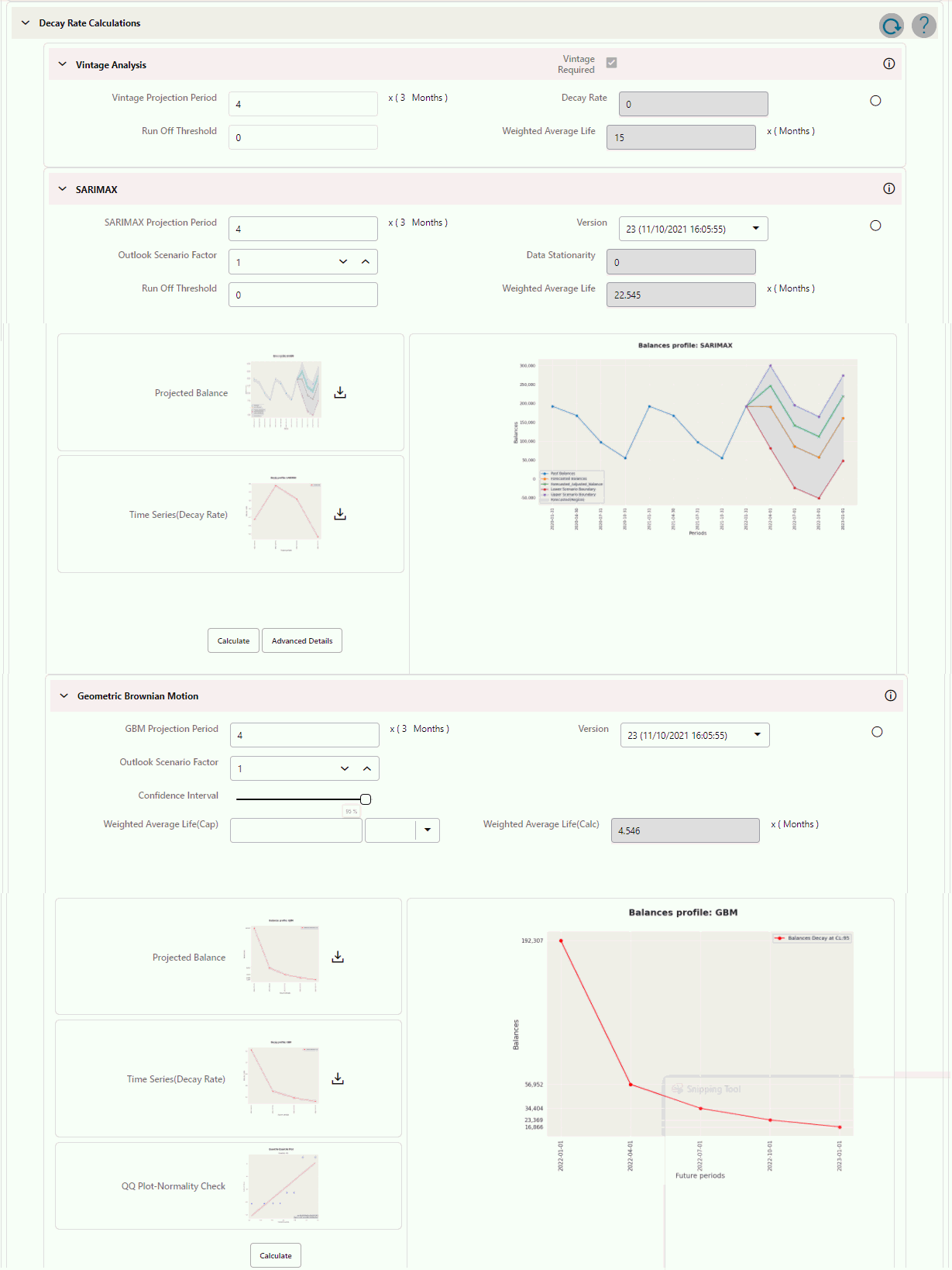    For Decay rate calculations, you can choose any one of following three approaches:

    • Vintage Analysis
    • SARIMAX
    • Geometric Brownian Motion

    Vintage Analysis: This method calculates one decay rate value as per the various vintages and regular intervals over which data is being picked for the defined portfolio. The same decay rate is applicable to the whole projection period. Select Vintage Analysis checkbox if you want to use this in calculation or exclude it from calculations. Vintage analysis needs account-level data for complete historical period, which you may not have initially, so you can avoid this method. For other methods, portfolio/cohort level data is required which is comparatively easier to get. By default, this checkbox is not selected to indicate this model is not included in processing. . You can set the projection period as per your requirement.

    SARIMAX: This method creates a future balance profile based on historical balances, along with Run-off volatility multiplied by the Outlook scenario factor (default 1). Based on balance Run-offs, a decay profile is created.

    Geometric Brownian Motion: Based on balance Run-off volatility and accepted user inputs like confidence interval and outlook scenario factor, Decay Rates are calculated for each subsequent period in projection period and decay profile is created.

    Based on the Decay Rate Profile, Run-offs would be calculated and finally, a balance profile will be created which will in turn help to calculate WAL.

    Based on the Decay Rates profile, the model will do Weighted Average Life (WAL) calculations as well, if WAL is more than defined regulatory WAL (Cap), then the system will let the user define a confidence interval range

    Figure 24-9 Confidence Interval Range

    
    

    

    
    

    and steps (Default 5%) in which confidence interval will be increased for each calculation. If the range is 80-95%, then the system generates a Decay Rate Profile at 80%, 85%, 90% and 95% interval; using an iterative process, try to calculate a Decay Rate Profile which will give WAL within regulatory WAL (Cap) defined by the user. If in a given confidence interval range, WAL is still more than regulatory WAL (Cap), a simple linear Decay Rate Profile would be created.

    Run-off threshold is a user input, it will define the minimum balance beyond which WAL calculations would not be performed, considering balance become zero at that point.

    When this window is launched first time and you press Calculate, Decay Rate is calculated for all three methods, Vintage Analysis, SARIMAX and Geometric Brownian Motion. After first run (when Calculate button does not appear), separate calculate buttons (as shown with SARIMAX and Geometric Brownian Motion) are available for each of Geometric Brownian motion and SRIMAX.

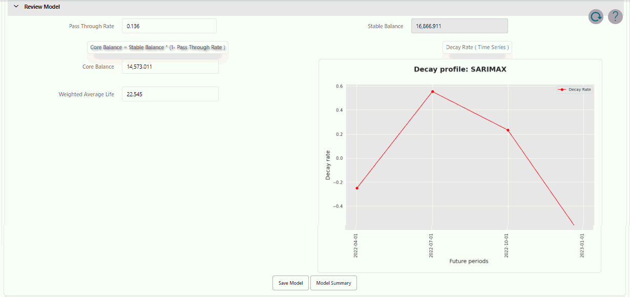
12. Click Next to navigate to the Review Model Section. This section shows the Model details before confirming the model. Here, you cannot edit any details. If you want to update any details, click Model Summary to go back. Until model is saved, it is always be in Draft status. It converts to Complete only when you save the model. For more information on editing, see the Editing Non-Maturity Products Model Analysis Rule section.

    Figure 24-10 Review Model section