Creating Non-Maturity Products Model

Step 1: Model Details

From Non-Maturity Products Model Analysis , click Start. The Model Details page is displayed.

Figure 6-282 Model Details
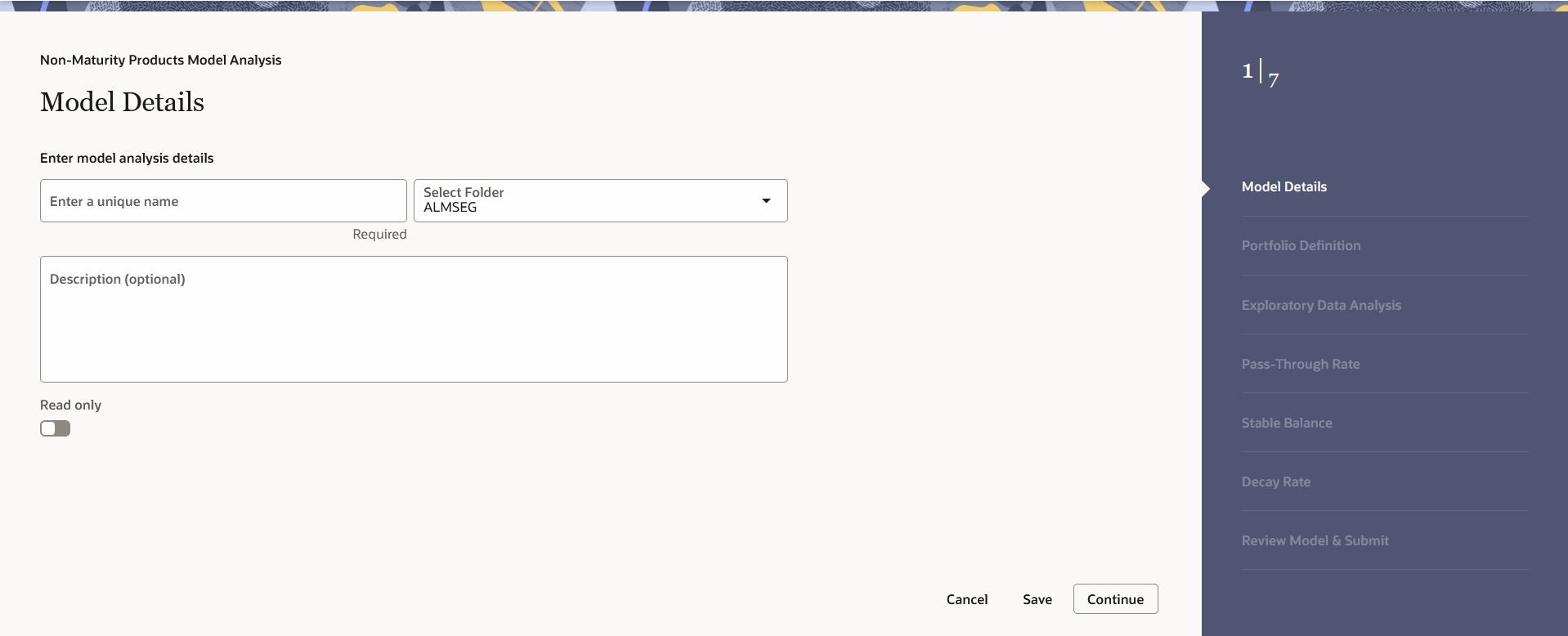
Enter the following details:
- Name: Name of model. The Non-Maturity Products Model name should be unique. Any special characters are not applicable.
- Folder: Folder Name where you want to save the model.
- Description: Description of model. The maximum limit of this field is 300 characters. You can enter special characters in this field.
Click Continue.

Step 2: Portfolio Selection

The Portfolio Selection window is displayed to set Portfolio.

Figure 6-283 Portfolio Selection

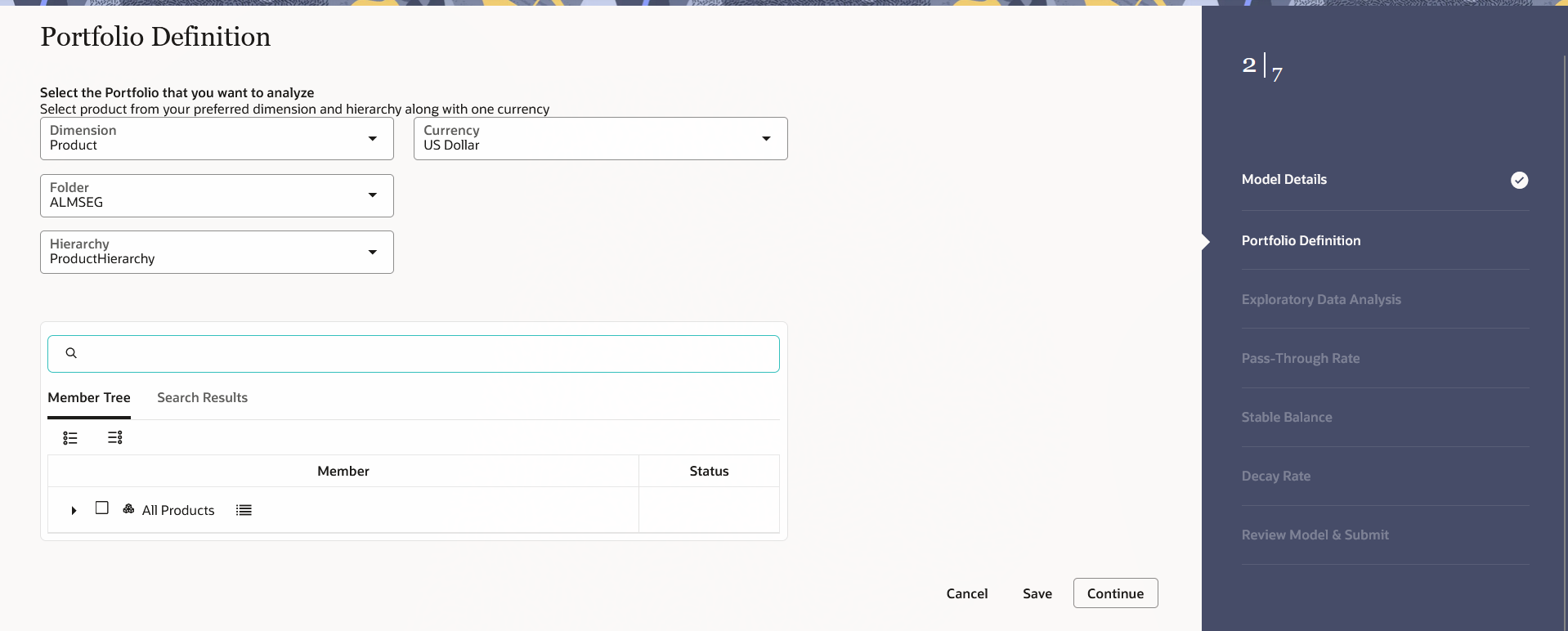
Enter the following details in Portfolio Selection section:
- Dimension: Select the dimension.
- Currency: Select the currency. The Currency drop-down displays the list of active currencies.
- Folder: Select the folder from which you want to pick the Hierarchy.
- Hierarchy: You can specify some parameters at product-currency combination. Hierarchies of selected folder will be listed and you can select one from the available list of hierarchies.
- Select Product(s) from Member Tree of Assumption Browser. The Assumption Browser has following two tabs: Member Tree and Search Results
  - Member Tree: Member Tree tab shows the hierarchical structure and allows you to define rules by selecting the node members from the browser. Select Node and Click Menu icon next to it to view the available options.
    
    Figure 6-284 Member Tree
    
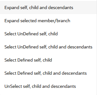
    Status of node is also displayed in Member Tree section, for example Selected, and so on. To select member hierarchy, following options are available:
    - Expand self, child and descendants: Allows to expand the selected node itself along with its child and descendants.
    - Expand selected member/branch: Allows to expand the selected node
    - Select UnSelect self, child: Allows to unselect the selected node itself along with its child
    - Select UnSelect self, child and descendants: Allows to unselect the selected node itself along with its child and descendants.
    - Select Defined self, child: Allows to select the selected node itself along with its child.
    - Select Defined self, child and descendants: Allows to select the selected node itself along with its child and descendants.
    - UnSelect self, child and descendants: Allows to unselect the selected node itself along with its child and descendants.
    Use Show Numeric Code Values (Left) icon to view the code value left to the Node name.
    
    Use Show Numeric Code Values (Right) icon to view the code value right to the Node name.
    
    Here, you can perform the following tasks on the selected node(s):
    - Add
    - Edit
    - View
    - Delete
    - Copy
  - Search Results: You can also search the members based on the filters. This section shows the searched node(s). To search a member, follow these steps:
    1. Navigate to Assumption Browser section of the Rule Definition page.
    2. Enter the Member ID, Name, Status, or Is Leaf in Search Criteria.
      
      Figure 6-285 Search Criteria
    3. Click Search. The searched member(s) will be displayed in Search Results section of Assumption Browser.
      
      Figure 6-286 Searching Members
      
      Here, you can perform the following tasks on the searched node(s):
      - Add
      - Edit
      - View
      - Delete
      - Copy
    Click Show Parentage icon to view the Parent-child Node level hierarchy details of selected Node.
    
    Use Show Numeric Code Values (Left) icon to view the code value left to the Node name.
    
    Use Show Numeric Code Values (Right) icon to view the code value right to the Node name.
Click Continue to navigate to Exploratory Data Analysis section.

Step 3: Exploratory Data Analysis

The Exploratory Data Analysis window is displayed to define Market Rates. This window will help you to perform EDA calculations and get a glimpse of data being used for modelling.

Figure 6-287 Exploratory Data Analysis

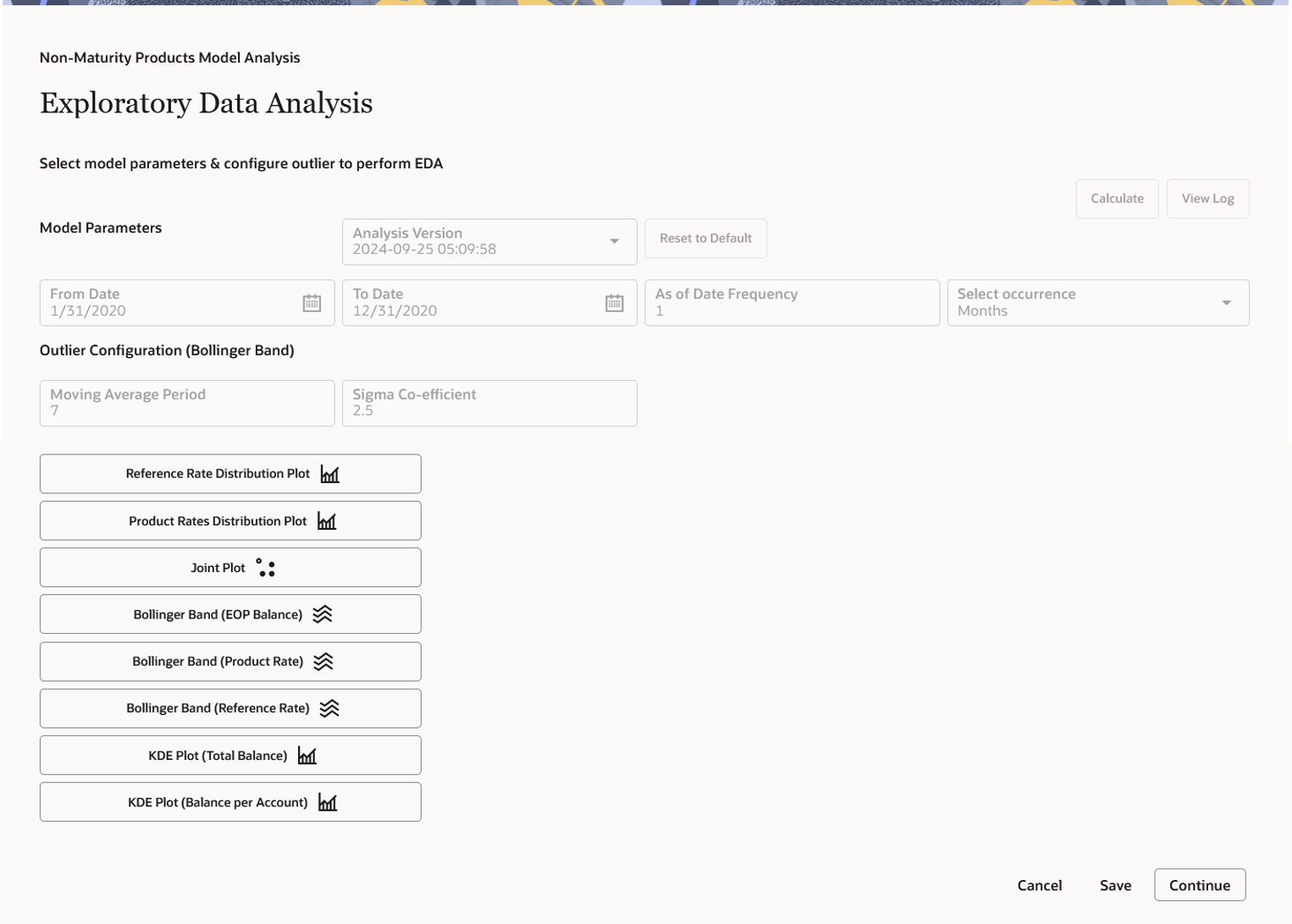
Enter the following details in the Exploratory Data Analysis section:
- Model Parameters (As of Date Range):
  - Analysis Versions: Shows the analysis version.
  - Model Parameters (As of Date Range): You can select a date range which will define the historical period within which data needs to be picked for Model creation. By default, the Date range is populated as below:
    - From Date: Max (As of Date) available in Model input Table.
    - To Date: Max [min (As of Date), From Date – 10 Years].
    Default values are populated from FSI_AUDIT_NM_LOAD_BATCH table.
  - As of Date Frequency: The default value of this field is one month. The As of Date Frequency defines on what regular intervals, data needs to be picked from the input table. For example, you can have historical period as last three years, in those three years at what regular interval data needs to be picked up from history table that would be defined by As of Date Frequency.
- Outlier Configuration (Bollinger Band):
  - Moving average period: The default value of this field is one month. The Moving Average period defines the historical term over which the moving average needs to be calculated for Bollinger band formation. This defines the period over which moving average gets calculated to create bollinger band.
  - Sigma Co-efficient: The default value of this field is 1. Sigma Co-efficient defines the outliers, any number which is (sigma coefficient * standard deviation) away from the mean, will not be considered for calculations. This field accepts Integer and Decimal values in the range 0 – 10. Sigma Co-efficients helps you to define the lower and upper bands for bollinger band graphs.
Click Calculate to perform Exploratory Data Analysis and get EDA plots. You can refresh the window using the Reset to Default button to check if the EDA is completed. When you open EDA window first time for a particular model, Version(EDA) field would not appear as there is no previous version to display. Subsequently, when first version is created and you go for second version, version (EDA) tab will start appearing with previous EDA versions. When EDA version is submitted, a message will appear with version number. A message is displayed in case last run version was failed. If run was successful and you again check this, the latest version would appear on the UI. The Reset to Default button resets the entered values to their default values.
Click Continue to navigate to Pass-Through Rate section.

Step 4: Pass-Through Rate

Pass Through Rate is based on linear regression between market and offered rate. For current accounts, the offered rate can be zero. In such cases, the pass-through rate will also be zero, as changes in the market rate do not affect the offered rate.

Figure 6-288 Pass-Through Rate

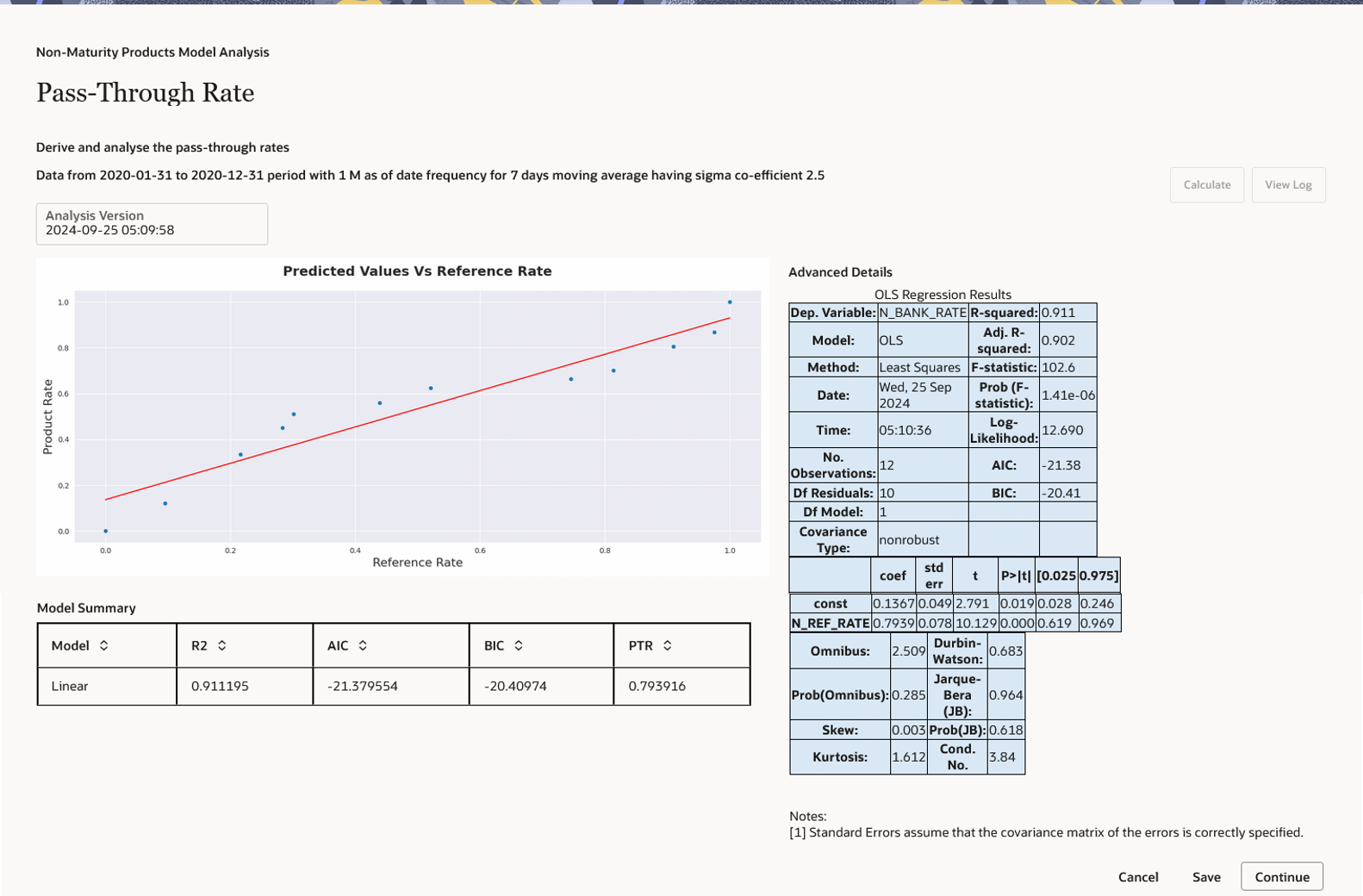
Click Calculate to view all the evaluation parameters and quality plots. Pass Through Rate calculations are submitted, a message is displayed with version number. This window shows all the model quality parameters and graphs. At this stage, Pass through rate or beta between market rate and deposit rate is calculated. You can zoom the graph to enhance visibility.
The Advanced Details section helps you to evaluate the model fit.

The Model Summary section shows the details of Model parameters like R2, AIC, BIC and regression co-efficient. That is, how much change in market rate is passed on to the deposit rate.

At any stage, if you want to come out of the model analysis module, click Cancel or Save button to go back to Non-Maturity products model summary screen.
Click Continue to navigate to Stable Balance section.

Step 5: Stable Balance

The Stable Balance section shows the Projection period.

Figure 6-289 Stable Balance

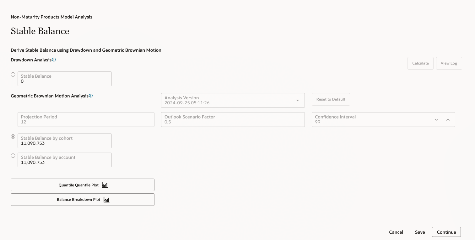
You can set the stable balance as required. Projection period can be only be positive integers which will act as multiplier to As of Date Frequency, for example, As of Date. To calculate Stable Balance, you can use following methods:
- DrawdownAnalysis: TheDraw Down Analysis calculates each period’s Run-offs in the historical period and subtracts the maximum Run-off from the most recent total balance to arrive at stable balance. This model performs calculations based on maximum Drawdown between two data points for given period.
  For example, analysis is done over past 5 years and monthly data points are given. If Balance is available for each data point, then system calculates balance reduction for each data point from previous data point. Finally, whatever will be the maximum balance reduction in two adjacent data points that is subtracted from point in time balance (Balance on latest As of Date) and remaining balance is the stable balance.
- Geometric Brownian Motion: This approach will first calculate the past Run-offs volatility and assuming normal distribution of Run-offs, accept confidence interval as user input, projection period for time adjustment, and outlook scenario factor (volatility multiplier) as input from the user.
  This model works based on historical volatility and confidence interval selected in the UI. It assumes that the underlying data follows a normal distribution, and based on the confidence interval, X% of the balance lies within the specified range. This allows the system to determine the stable balance.
  
  95% Confidence Interval – (-1.96 to +1.96)
  
  90% Confidence Interval – (-1.645 to +1.645)
  
  80% Confidence Interval – (-1.282 to +1.282)
  
  Here, you can select the outlook scenario factor, which will be multiplied with historical volatility and subsequently used for Geometric Brownian Motion based stable balance calculations.
  
  Geometric Brownian Motion outcome is based on both portfolio level balance volatility and account level balance volatility. You can select any of the stable balances, which are more suitable as per the given context.
The confidence interval slider field has a range of 0 – 100% and by default value as 95% and Outlook scenario factor (Volatility Multiplier) is set at 1 (Default Value). The range of outlook scenario factor is 0.01 to 1.99.

You can change any of the inputs and generate multiple versions.
After clicking Calculate, the stable balance would be shown at cohort/account level using both cohort level and account level volatility and saved against version.
Stable balance can be calculated with multiple methods, so before proceeding to next step, you must select Stable Balance by Cohot or Stable Balance by account method to confirm one stable balance on which rest of the subsequent processing will take place.

When this section is displayed first time, after clicking the Calculate, the stable balance is calculated for both methods, Drawdown analysis and Geometric Brownian Motion.

In subsequent runs, if any of projection period, confidence interval or Scenario factor is changed, then new version will be generated only for Geometric Brownian Motion. When you click Calculate button, then a message is displayed: GBM version xyz is submitted. If version is failed, a message is displayed: GBM version xx is failed and UI will revert back to last successful version.
Click Continue to navigate to Decay Rate section.

Step 6: Decay Rate

For Decay rate calculations, you can select any one of following three approaches:

Vintage Analysis
SARIMAX
Geometric Brownian Motion

Figure 6-290 Decay Rate

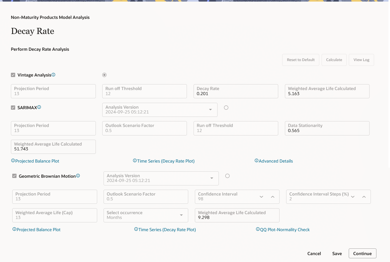
Select the Decay Rate method:
- Vintage Analysis: This method calculates one decay rate value as per the various vintages and regular intervals over which data is being picked for the defined portfolio. The same decay rate is applicable to the whole projection period.
  The vintage run-off model aims to categorize deposit balances based on historical tranches, referred to as vintages. A vintage comprises all individual accounts for a non-maturing deposit account type that were opened within a specific time bucket, such as a month or week. Behavioral characteristics are applied to each vintage by calculating the monthly decay within each vintage. Run-off calculations are performed across data points and account origination buckets, with the final decay rate being the average of both dimensions for the selected portfolio.
  
  Select the Vintage Analysis check-box if you want to include it in the calculation, or leave it unchecked to exclude it. Vintage analysis requires account-level data for the entire historical period, which may not be available initially, so you can opt to bypass this method. Other methods use portfolio or cohort-level data, which is generally easier to obtain. By default, the check-box is unchecked, indicating that this model is not part of the processing. You can set the projection period according to your needs.
- SARIMAX: This method creates a future balance profile based on historical balances, along with Run-off volatility multiplied by the Outlook scenario factor (default 1). Based on balance Run-offs, a decay profile is created.
  Among the various approaches, the SARIMAX model (Seasonal Autoregressive Integrated Moving Average with exogenous variables) is a powerful tool for modeling and forecasting trends and seasonal variations in time series data. It also incorporates external variables to enhance prediction accuracy. This model is part of the ARIMA family and is built on three key components: autoregression (AR), moving average (MA), and integration (I).
  - Autoregression (AR) uses past values of the time series to predict the current value.
  - Moving average (MA) accounts for past prediction errors, applying a linear regression on the last "q" error values to forecast the present.
  - Integration (I) makes the data stationary by accounting for differences between consecutive observations.
  For data with seasonal variations, the SARIMA model is used, adding the "Seasonal" component to ARIMA, which captures patterns that repeat at regular intervals. Based on the decay rate in each period, the weighted average life is calculated by multiplying the run-off matrix with the time series.
- Geometric Brownian Motion: Based on balance Run-off volatility and your inputs like confidence interval and outlook scenario factor, the Decay Rates are calculated for each subsequent period in projection period and decay profile is created. Based on the Decay Rate Profile, Run-offs would be calculated and finally, a balance profile will be created which will in turn help to calculate WAL.
  Based on the Decay Rates profile, the model will do Weighted Average Life (WAL) calculations. If the WAL exceeds the specified regulatory cap, you can set a confidence interval range and steps (defaulting to 5%) for adjusting the confidence interval in each calculation. For example, if the range is 80-95%, the system will generate a Decay Rate Profile at 80%, 85%, 90%, and 95% intervals. Through an iterative process, it will attempt to calculate a Decay Rate Profile that brings the WAL within the regulatory cap set by the user.
  
  If in a given confidence interval range, WAL is still more than regulatory WAL (Cap), a simple linear Decay Rate Profile is created.
  
  The run-off threshold is a user-defined input that sets the minimum balance at which WAL calculations will stop, assuming the balance has reached zero at that point.
Note:
When this section is launched first time and you click Calculate, Decay Rate is calculated for all three methods, Vintage Analysis, SARIMAX, and Geometric Brownian Motion.
Click Continue to navigate to Review and Submit section.

Step 7: Review and Submit

Navigate to Preview and Submit section. This section shows the Model details before confirming the model. Here, you cannot edit any details. If you want to update any details, click Model Summary to go back. When model is saved, it is always be in Draft status.
Click Submit to create the Non Maturity Products Model. The created process will be displayed on Non Maturity Products Model Summary page.

6.4.1.1 Creating Non-Maturity Products Model