6.5.4 Shock Types for Variables

Shock Type for numeric variables

If you have selected numeric type of variable select from one of the shock type and provide your inputs.

Note:

For MEVTS variables, only the following shock types are applicable:

• Absolute Values
• Constant Absolute Growth per Annum
• Constant Growth in Percentage per Annum

• Absolute Value - the formula to calculate this is:
  
  
  
  

  Where,

  Input Value is the value entered on the User Interface (UI).

• Absolute Growth on Current value (AGC) - the formula to calculate this is:
  
  
  
  

  Where,

  Current Value - is the reference value entered on the UI

  Input Grid Value - percentage or absolute value you enter by which you want to increase or decrease the current value of reference date.

• Absolute Growth on Future value (AGF) - the formula to calculate this is:
  
  
  
  

  Where,

  *For each iteration the Current Value is updated based on the previous calculation.

  Current Value - is the reference value entered on the UI

  Input Grid Value - is the percentage or absolute value you enter by which you want to increase or decrease the current value of reference date.

• Constant Absolute Growth Per Annum (CAGPA) - the formula to calculate this is:
  
  
  
  

  Where,

  Current Value - is the reference value entered on the UI

  Input Percentage - is the percentage value of growth or deprecation

  Date Difference - is the frequency selected.

• Constant Growth in Percentage Per Annum (CGPPA) - the formula to calculate this is:
  
  
  
  

  Where,

  Current Value - is the value entered on the UI.

  Input Percentage - is the percentage value of growth or deprecation

  Date Difference - is the frequency for the calculations

• Percentage Growth Per Annum over Current Value (PGPAC) - the formula to calculate this is:
  
  
  
  

  Where,

  Current Value - is the value entered on the UI.

  Input Grid Percentage - is the percentage you enter by which you want to increase or decrease the current value of reference date.

• Percentage Growth Per Annum over Future value (PGPAF) - the formula to calculate this is:
  
  
  
  

  Where,

  *For each iteration the Current Value is updated based on the previous calculation

  Input Grid Percentage - is the change per annum

  Data Difference - is the difference between the frequency of dates mentioned

Examples of Shock Types

Below is a list of examples for all the shock types with details:

For example, you enter the following values in the Time Horizon Details section of the scenario wizard:

Frequency: monthly

Time Frame: 2

Reference Date: 21/May/2024

Start Date: 31/May/2024

For Absolute Value shock type, the calculations are as follows:

1. The start date is displayed as part of the first sequence that is 31/May/2024 and the next date is calculated based on the frequency type (in this case, monthly or 30 days difference). Hence, the next date is 30/June/2024.
2. In this case, you can define the current value and the absolute values for the variables on 31^st may and 30^th June as 10, 50 and 10.

For Absolute growth on Current value shock type, the calculations are as follows:

1. The start date is displayed as part of the first sequence that is 31/May/2024 and the next date is calculated based on the frequency type (in this case, monthly or 30 days difference). Hence, the next date is 30/June/2024.
2. In this case, you can define the current value and the absolute values for the variables on 31^st may and 30^th June as 10, 50 and 10.
3. When you click Compute input values, then the growth on the absolute values for 31^st may and 30^th June are 60 and 20.
   Since,

   • Absolute Growth on Current value on 31/May/2024 (60) = Current Value (10) + Input Value on 31/May/2024 (50)
   • Absolute Growth on Current value on 30/June/2024 (20) = Current Value (10) + Input Value on 30/June/2024 (10)

For Absolute growth on future value shock type, the calculations are as follows:

1. The start date is displayed as part of the first sequence that is 31/May/2024 and the next date is calculated based on the frequency type (in this case, monthly or 30 days difference). Hence, the next date is 30/June/2024.
2. In this case, you can define the current value and the absolute values for the variables on 31^st May and 30^th June as 10, 50 and 10.
3. When you click Compute input values, then the growth on the absolute values for 31^st May and 30^th June are 60 and 70.
   Since,

   • Absolute Growth on future value on 31/May/2024 (60) = Current Value (10) + Absolute Value (or Input Value) on 31/May/2024 (50)
   • Absolute Growth on future value on 30/June/2024 (70) = Current Value (60) + Absolute Value (or Input Value) on 30/June/2024 (10)

For Constant absolute growth per annum shock type, the calculations are as follows:

1. The start date is displayed as part of the first sequence that is 31/May/2024 and the next date is calculated based on the frequency type (in this case, monthly or 30 days difference). Hence, the next date is 30/June/2024.
2. In this case, you can define the Absolute value or Constant Absolute Value(FOR ALL DATES) percentage as 50% and the Current Value as 10.
3. When you click Compute input values, then the absolute growth for 31^st May and 30^th June are 11.3889 and 15.5556.
   Since,

   • DDC1: Date Difference From Current Value (D1-D0)=10

     DDC2: Date Difference From Current Value(D2-D0)=40

   • Constant Absolute Growth Per Annum on 31/May/2024 (11.3889) = 10 +(50*(10/360))
   • Constant Absolute Growth Per Annum on 30/June/2024 (15.5556) = 10+(50*(40/360))

For Constant growth in percentage per annum shock type, the calculations are as follows:

1. The start date is displayed as part of the first sequence that is 31/May/2024 and the next date is calculated based on the frequency type (in this case, monthly or 30 days difference). Hence, the next date is 30/June/2024.
2. In this case, you can define the percentage or the Constant Percentage Value as 50% and current value as 10.
3. When you click Compute input values, then the growth rate on 31^st May and 30^th June are 10.1133 and 10.4608.
   Since,

   • DDC1: Date Difference From Current Value (D1-D0)=10

     DDC2: Date Difference From Current Value(D2-D0)=40

   • Constant growth in percentage per annum on 31/May/2024 (10.1133) = 10*(1+(50/100))^(10/360)
   • Constant growth in percentage per annum on 30/June/2024 (10.4608) = 10*(1+(50/100))^(40/360)

For Overall Percentage Growth over current value shock type, the calculations are as follows:

1. The start date is displayed as part of the first sequence that is 31/May/2024 and the next date is calculated based on the frequency type (in this case, monthly or 30 days difference). Hence, the next date is 30/June/2024.
2. In this case, you can define the current value and the growth over current value percentages on 31st may and 30th June as 10, 50% and 10%.
3. When you click Compute input values, then the growth rate on 31^st May and 30^th June are 10.1133 and 10.1065.
   Since,

   • DDC1: Date Difference From Current Value (D1-D0)=10

     DDC2: Date Difference From Current Value(D2-D0)=40

   • Percentage Growth per annum over future value on 31/May/2024 = 10*(1+50/100)^(10/360)
   • Percentage Growth per annum over future value on 30/June/2024 = 10*(1+10/100)^(40/360)

For Percentage Growth per annum over future value shock type, the calculations are as follows:

1. The start date is displayed as part of the first sequence that is 31/May/2024 and the next date is calculated based on the frequency type (in this case, monthly or 30 days difference). Hence, the next date is 30/June/2024.
2. In this case, you can define the current and the growth over future percentages on 31^st may and 30^th June as 10, 50% and 10%.
3. When you click Compute input values, then the growth rate on 31^st May and 30^th June are 10.1133 and 10.1939.
   Since,

   • Overall Percentage Growth over current value on 31/May/2024 = 10*(1+(50/100))
   • Overall Percentage Growth over current value on 30/June/2024 = 10*(1+(10/100))

Categorical Shock Type

If you have selected categorical type of variable select from one of the shock type and provide your inputs:

• Change of Class - based on the frequency entered you can select the value for this variable from the existing values
• Constant Notch Up/Down on Current Value - based on the current value, the variable value is increased or decreased by a notch.
• Constant Notch Up/Down on Future Value - based on the value entered, the next value that is the future value is calculated by increasing or decreasing the value by a notch (or by one value).
• Notch Up/Notch Down on Current Value - based on the current value, the variable value is increased or decreased by a notch (or by one value).
• Notch Up/Notch Down on Future Value - based on the value entered, the next value that is the future value is calculated by increasing or decreasing the value by a notch (or by one value).

• Universal
  • When dimension is added to the selected variable- the grid maps each node in the dimension. Your input for each dimension node impacts all variable hierarchy nodes within that specific dimension node.
  • When there are no dimensions in the selected variable - there is a single row of mapping for each variable hierarchy. Your input for that row affects all the nodes within the variable hierarchy.
• Local
  • When dimension is added to the selected variable- the grid maps each node in the variable hierarchy to every node in the dimension.
  • When there are no dimensions in the selected variable - the grid maps each node within the variable hierarchy individually.

Shock Type for MEVTS variable

This is a numerical variable with either a Micro or Macro subtype. Additionally, the tsBased flag is enabled, which allows the variable to capture its frequency, timeframe, and the start/end of the period during its creation.

Table 6-7 Scenario Grid Generation

Country	Observation Date	CV	03-06-2025	03-07-2025	03-08-2025
India	30-04-2025	5%	4.75%	4.75%	4.75%
India	31-07-2025	5%	4.50%	4.50%	4.50%
India	31-10-2025	5%	4.25%	4.25%	4.25%
India	31-01-2026	5%	4.00%	4.00%	4.00%
India	30-04-2026	5%	3.75%	3.75%	3.75%
India	31-07-2026	5%	3.50%	3.50%	3.50%
US	30-04-2025	5%	4.75%	4.75%	4.75%
US	31-07-2025	5%	4.50%	4.50%	4.50%
US	31-10-2025	5%	4.25%	4.25%	4.25%
US	31-01-2026	5%	4.00%	4.00%	4.00%
US	30-04-2026	5%	3.75%	3.75%	3.75%
US	31-07-2026	5%	3.50%	3.50%	3.50%

• Observation Date Calculation
  The Observation Date column is unique to MEVTS variables and is calculated as follows:

  • The first observation date is set as the scenario reference date.
  • The total number of observation dates is equal to the variable's timeframe.
  • The interval between observation dates is determined by the variable's frequency.
  • The Start-of-Period / End-of-Period setting determines whether the observation dates align with the beginning or end of each period.

Shock Types for MEVTS Variables

Three types of shocks are supported:

• Absolute Values: Users manually input absolute values in the scenario grid.

  Figure 6-1 MVETS Absolute Values

  
  

  

  
  
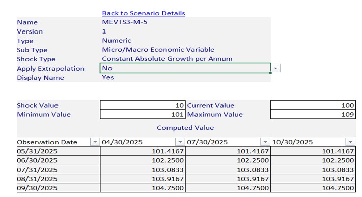
• Constant Absolute Growth per Annum:

  The formula and other configurations remain unchanged. However, in this case, the values are calculated based on observation dates corresponding to future periods. Minimum and maximum bounds are also applied for time series (TS)-based variables.

  For example, if the user provides a current value of 5%, the calculation for the first future date (for example, 03/06/2025) will be based on the observation period from 30/04/2025 to 31/05/2025.

  For the next future date (03/07/2025), the value from 03/06/2025 will be carried forward through interpolation, which, in this case, remains unchanged. As a result, the values across all future dates remain consistent, as shown in the scenario grid.

  Figure 6-2 Constant Absolute Growth per Annum

  
  

  

  
  

  Extrapolation Support

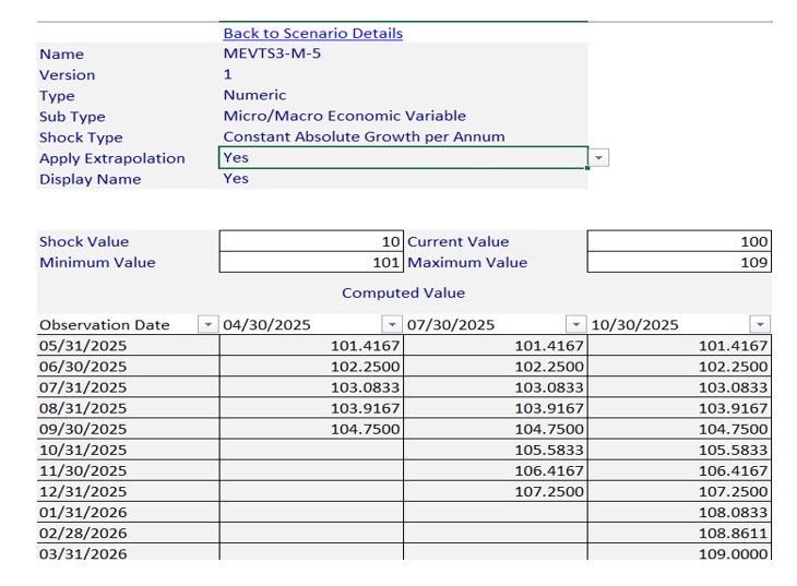
  Users can enable extrapolation to extend observation dates beyond the current timeframe.

  • A new grid appears with extended future dates.
  • The number of extra dates depends on the frequencies of the scenario and the variable.
  Frequency Base Days:

  • Yearly (Y): 360 days
  • Quarterly (Q): 90 days
  • Monthly (M): 30 days
  • Weekly (W): 7 days
  • Daily (D): 1 day

  The formula to calculate this is:

  Figure 6-3 MVETS Variable formula

  
  

  

  
  

  Example:

  If the scenario frequency is Quarterly (90 days) and the variable frequency is Monthly (30 days):

  Q/M = 90/30 = 3, therefore, 3 new dates are added per extrapolation step.

  Extrapolated values are calculated using the same formula as defined for the selected shock type.

  Figure 6-4 MVETS Variable Example

  
  

  

  
  
• Constant Growth in Percentage per Annum:

  This type follows the same rules as the Constant Absolute Growth per Annum shock type, but uses a percentage-based growth formula.

Additional Information

• Interpolation (in Finance)

  Used to estimate values within the range of known data points.

  Example:

  If a bond yields 4% for a 1-year maturity and 6% for a 3-year maturity, interpolation can estimate the 2-year yield.

• Extrapolation (in Finance)

  Used to estimate values beyond the range of known data points based on trends.

  Example:

  If a stock grows 10% per year over 3 years, extrapolation can estimate its price in the next year, assuming the trend continues.

Shock Types for IRC Variables

If you have selected numeric type of variable select from one of the shock type and provide your inputs.

• Absolute Value - the formula to calculate this is:
  
  
  
  

  Where,

  Input Value is the value entered on the User Interface (UI).

• IRC Variable Grid Formation

  During the variable creation process, terms and multipliers are defined for the IRC variable.

  Users can then enter current values, and the system will calculate corresponding future date values.

  The resulting grid appears as follows:

  Figure 6-5 IRC Variable Grid Formation

  
  

  

  
  

  IRC variable also has absolute value shocktype.

• Flat:: the formula to claculate this is as follows:

  Figure 6-6 IRC Variable Grid Formation

  
  

  

  
  

  In this shock type, the user provides input only for the current value.

  All future values remain unchanged, resulting in a flat curve with no variation across time.

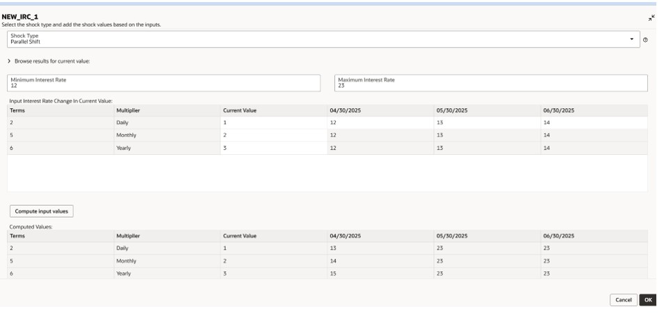
• Parallel Shift: the formula to claculate this is as follows:

  Figure 6-7 Parallel Shift formula

  
  

  

  
  

  The user may optionally specify minimum and maximum bound values.

  A single delta value is entered for all future dates and is uniformly applied to the current values.

  This results in a parallel shift of the entire curve.