What Is State Estimation
State estimation utilizes a Weight Least Squares algorithm. This is a non-linear least squares solver. We build up a system of equations that fall into one of four types:
1. Measurement Residuals: The individual measurements we have. These are simple (Measurement Value – Estimated Value)
2. Zero-Injection Residuals: Enforce Kirchhoff's Current Law by requiring the sum of complex current into a zero-injection node to be zero.
3. Pseudo-Measurement Residuals: Compare calculated complex current injection with the expected injection derived from modeled load, generation, or capacitor values. These residuals use separate uncertainty settings because the expected injection is less certain than a direct measurement.
4. Voltage-Equality Residuals: For selected phases across high-admittance, low-impedance pass-through branches, require the complex voltages on the two connected nodes to be equal. These residuals use the voltage-equivalence uncertainty configured by rule value 2 of DSE_HIGH_ADMITTANCE_TOL.
The goal of state estimation is to find a “best estimate” of nodal voltages: Vi that minimizes a weighted least squares equation constructed from those 3 different residual equations above. Assume we have M measurements for N nodes. Each specific measurement (for a device and measurement type) has a computable estimate: Est(V) that depends on the state of the network (that is voltages at multiple nodes). For given set of voltages V, we can compute the (complex) power in each individual branch: Sbr(V). Taken together we seek to minimize a function f(V) that is defined by:
f(V) = sum from i=0 to M of W_i^2 [Meas_i - Est_i(V)]^2
+ sum from j=0 to N of W_j^2 |I_j_expected - I_j(V)|^2
+ sum from k=0 to L of W_k^2 |V_from,k - V_to,k|^2
Where M is the set of telemetry measurement residuals, N is the set of zero-injection and pseudo-measurement current residuals, and L is the selected set of voltage-equality residuals across low-impedance pass-through branches. Represent the current and voltage-equality terms as separate real and imaginary residual rows, or equivalent complex-magnitude notation.
Est(V) is one of the following functions: Voltage, Angle, Current, Real Power, or Reactive Power. The computation of it changes by each type. The individual weights have a large impact on results. Each measurement can define its own weight. We define weight in terms of expected measurement errors (variance/standard deviation). These are computed assuming two independent forms of error: Relative Error and Absolute Error as follows:
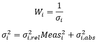
Which allows small measurements to be just as important as large measurements (note Meas used here is a per-unit measurement, and if σ is zero we disable the measurement).
For current-injection equations, DSE uses the configured pseudo-measurement uncertainty at nodes with modeled load, generation, or capacitors. At zero-injection nodes, the expected complex current is zero and DSE uses DSE_ZEROINJ_WEIGHT as the absolute uncertainty. Smaller uncertainty values give these current-balance constraints greater influence. DSE normalizes weights internally for solver stability, but user-facing weights remain on their physical 1/sigma scale.
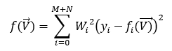
Which is in the standard form of a non-linear least squares. We solve this via iteratively reweighted least squares with Levenberg-Marquardt (damped least squares), meaning the non-linear solver can reweight residuals to reduce the impact of outliers, these are applied on top of the configured weights.