- Generate demand forecasts at scale using Oracle Cloud Infrastructure
- Generate Demand Forecasts
Generate Demand Forecasts
These steps describe how to generate demand forecasts in your OCI Data Science notebook.
Set Up Environment
- On the data science notebook, setup the OCI Data Flow session. Use the
pip install prophetpython library when building your custom conda package.import ads ads.set_auth("resource_principal") %reload_ext dataflow.magics %help import json command = { "compartmentId": "your-compartment-ocid", "displayName": "display-name", "sparkVersion": "3.2.1", "driverShape": "VM.Standard.E3.Flex", "executorShape": "VM.Standard.E3.Flex", "driverShapeConfig":{"ocpus":1,"memoryInGBs":16}, "executorShapeConfig":{"ocpus":1,"memoryInGBs":16}, "numExecutors": 1, "metastoreId": "your-metastore-ocid", "configuration":{ "spark.archives":"oci://your-oci-bucket-name@your-oci-tenancy-name/your-custom-conda-env-path#conda", "spark.oracle.datasource.enabled":"true", "spark.delta.logStore.oci.impl":"io.delta.storage.OracleCloudLogStore", "spark.sql.extensions":"io.delta.sql.DeltaSparkSessionExtension", "spark.sql.catalog.spark_catalog":"org.apache.spark.sql.delta.catalog.DeltaCatalog"} } command = f'\'{json.dumps(command)}\'' print("command",command) - Import dependent python libraries. For example:
%%spark
#Import required libraries.

import json
import os
import sys
import datetime
import oci
import pyspark.sql
from pyspark.sql.functions import countDistinct

from pyspark.ml import Pipeline
from pyspark.ml.classification import DecisionTreeClassifier
from pyspark.ml.feature import StringIndexer, VectorIndexer
from pyspark.ml.evaluation import MulticlassClassificationEvaluator
# $example off$
from pyspark.sql import SparkSession

from delta.tables import *

import pandas as pd

from prophet import Prophet
import logging

import matplotlib.pyplot as plt
Examine Data
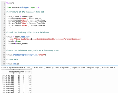
- Examine the data.For our training dataset, we will make use of five years of store item unit sales data for 50 items across 10 different stores.
%%spark from pyspark.sql.types import * # structure of the training data set train_schema = StructType([ StructField('date', DateType()), StructField('store', IntegerType()), StructField('item', IntegerType()), StructField('sales', IntegerType()) ]) # read the training file into a dataframe train = spark.read.csv( 'oci://demo-bucket@orasenatdpltintegration03/forecast/bronze/train.csv', header=True, schema=train_schema ) # make the dataframe queryable as a temporary view train.createOrReplaceTempView('train') # show data train.show() - View yearly trends when performing demand forecasting, we are often interested in general trends and seasonality. Let's start our exploration by examining the annual trend in unit sales.
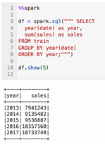
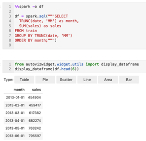
%%spark df = spark.sql(""" SELECT year(date) as year, sum(sales) as sales FROM train GROUP BY year(date) ORDER BY year;""") df.show(5)It's very clear from the data that there is a generally upward trend in total unit sales across the stores. If we had better knowledge of the markets served by these stores, we might want to identify whether there is a maximum growth capacity we'd expect to approach over the life of our forecast. Without that knowledge and by quickly seeing this dataset, it feels safe to assume that if our goal is to make a forecast a few days, months, or even a year out, we might expect continued linear growth over that time span. - View monthly trends.Let's examine seasonality. If we aggregate the data around the individual months in each year, a distinct yearly seasonal pattern is observed which seems to grow in scale with overall growth in sales.
%%spark -o df

df = spark.sql("""SELECT
  TRUNC(date, 'MM') as month,
  SUM(sales) as sales
FROM train
GROUP BY TRUNC(date, 'MM')
ORDER BY month;""")
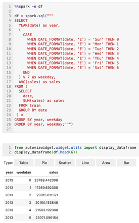
from autovizwidget.widget.utils import display_dataframe display_dataframe(df.head(6)) - View weekday trends.By aggregating the data at a weekday level, a pronounced weekly seasonal pattern is observed with a peak on Sunday (weekday 0), a hard drop on Monday (weekday 1) and then a steady pickup over the week heading back to the Sunday high. This pattern seems to be stable across the five years of observations.
%%spark -o df

df = spark.sql("""
SELECT
  YEAR(date) as year,
  (
    CASE
      WHEN DATE_FORMAT(date, 'E') = 'Sun' THEN 0
      WHEN DATE_FORMAT(date, 'E') = 'Mon' THEN 1
      WHEN DATE_FORMAT(date, 'E') = 'Tue' THEN 2
      WHEN DATE_FORMAT(date, 'E') = 'Wed' THEN 3
      WHEN DATE_FORMAT(date, 'E') = 'Thu' THEN 4
      WHEN DATE_FORMAT(date, 'E') = 'Fri' THEN 5
      WHEN DATE_FORMAT(date, 'E') = 'Sat' THEN 6
    END
  ) % 7 as weekday,
  AVG(sales) as sales
FROM (
  SELECT
    date,
    SUM(sales) as sales
  FROM train
  GROUP BY date
 ) x
GROUP BY year, weekday
ORDER BY year, weekday;""")
from autovizwidget.widget.utils import display_dataframe display_dataframe(df.head(6))
Generate a Single Forecast
Let's generate a single demand forecast before attempting to generate forecasts for individual combinations of stores and items. It might be helpful to build a single forecast for no other reason than to orient ourselves to the use of prophet.
- Our first step is to assemble the historical dataset on which we will train the model.
%%spark

history_pd = spark.sql("""
  SELECT
    CAST(date as date) as ds,
    sales as y
  FROM train
  WHERE store=1 AND item=1
  ORDER BY ds
""").toPandas()

history_pd = history_pd.dropna()

history_pd = history_pd.dropna()
Now, we will import the prophet library, but because it can be a bit verbose when in use, we need to fine tune the logging settings in our environment.%%spark from prophet import Prophet import logging # disable informational messages from prophet logging.getLogger('py4j').setLevel(logging.ERROR)%%spark # set model parameters model = Prophet( interval_width=0.95, growth='linear', daily_seasonality=False, weekly_seasonality=True, yearly_seasonality=True, seasonality_mode='multiplicative' ) # fit the model to historical data model.fit(history_pd) - Next, let's build a forecast.
%%spark -o df

# define a dataset including both historical dates & 90-days beyond the last available date
future_pd = model.make_future_dataframe(
  periods=90,
  freq='d',
  include_history=True
  )

forecast_pd = model.predict(future_pd)

df=spark.createDataFrame(forecast_pd)
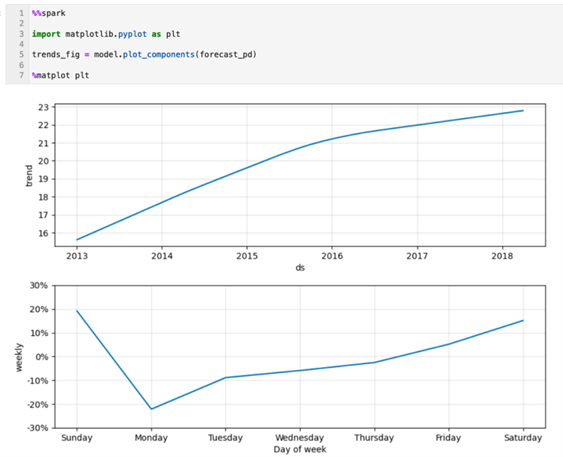
from autovizwidget.widget.utils import display_dataframe display_dataframe(df.head(6)) - Examine forecast components.How did our model perform? Here we can see the general and seasonal trends in our model presented as graphs.
%%spark import matplotlib.pyplot as plt trends_fig = model.plot_components(forecast_pd) %matplot plt - View historical data vs. prediction data.Here, we can see how our actual and predicted data line up as well as a forecast for the future, though we will limit our graph to the last year of historical data to keep it readable.
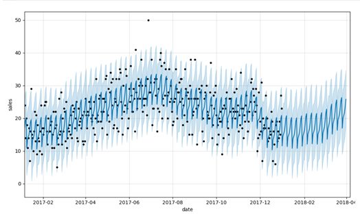
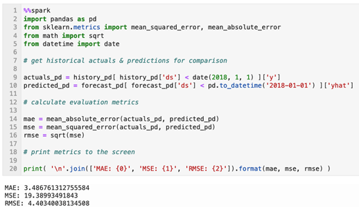
%%spark predict_fig = model.plot( forecast_pd, xlabel='date', ylabel='sales') # adjust figure to display dates from last year + the 90 day forecast xlim = predict_fig.axes[0].get_xlim() new_xlim = ( xlim[1]-(180.0+365.0), xlim[1]-90.0) predict_fig.axes[0].set_xlim(new_xlim) import matplotlib.pyplot as plt %matplot pltThis visualization is a bit busy. The black dots represent our actuals with the darker blue line representing our predictions and the lighter blue band representing our (95%) uncertainty interval. - Calculate evaluation metrics.Visual inspection is useful, but a better way to evaluate the forecast is to calculate Mean Absolute Error, Mean Squared Error, and Root Mean Squared Error values for the predicted relative to the actual values in our set.
%%spark
import pandas as pd
from sklearn.metrics import mean_squared_error, mean_absolute_error
from math import sqrt
from datetime import date

# get historical actuals & predictions for comparison

actuals_pd = history_pd[ history_pd['ds'] < date(2018, 1, 1) ]['y']
predicted_pd = forecast_pd[ forecast_pd['ds'] < pd.to_datetime('2018-01-01') ]['yhat']

# calculate evaluation metrics

mae = mean_absolute_error(actuals_pd, predicted_pd)
mse = mean_squared_error(actuals_pd, predicted_pd)
rmse = sqrt(mse)

# print metrics to the screen

print( '\n'.join(['MAE: {0}', 'MSE: {1}', 'RMSE: {2}']).format(mae, mse, rmse) )
Generate Forecasts at Scale
- Scale forecast generation.With the mechanics under our belt, let's tackle our original goal of building numerous, fine-grain models and forecasts for individual store and item combinations. We will start by assembling sales data at the store-item-date level of granularity. Retrieve data for all store-item combinations. The data in this data set should already be aggregated at this level of granularity, but we are explicitly aggregating to ensure we have the expected data structure.
%%spark sql_statement = ''' SELECT store, item, CAST(date as date) as ds, SUM(sales) as y FROM train GROUP BY store, item, ds ORDER BY store, item, ds ''' store_item_history = ( spark .sql( sql_statement ) .repartition(sc.defaultParallelism, ['store', 'item']) ).cache() - With our data aggregated at the store-item-date level, we need to consider how we will pass our data to prophet. If our goal is to build a model for each store and item combination, we will need to pass in a store-item subset from the dataset we just assembled, train a model on that subset, and receive a store-item forecast back. We'd expect that forecast to be returned as a dataset with a structure like this where we retain the store and item identifiers for which the forecast was assembled, and we limit the output to just the relevant subset of fields generated by the Prophet model.
%%spark from pyspark.sql.types import * result_schema =StructType([ StructField('ds',DateType()), StructField('store',IntegerType()), StructField('item',IntegerType()), StructField('y',FloatType()), StructField('yhat',FloatType()), StructField('yhat_upper',FloatType()), StructField('yhat_lower',FloatType()) ]) - To train the model and generate a forecast we will leverage a Pandas function. We will define this function to receive a subset of data organized around a store and item combination. It will return a forecast in the format identified in the previous cell.
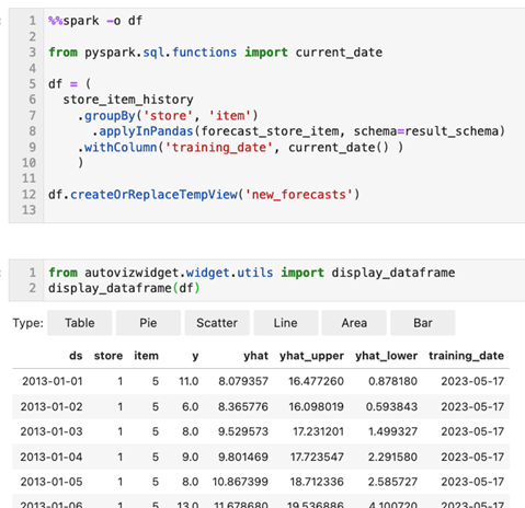
%%spark def forecast_store_item( history_pd: pd.DataFrame ) -> pd.DataFrame: # TRAIN MODEL AS BEFORE # -------------------------------------- # remove missing values (more likely at day-store-item level) history_pd = history_pd.dropna() # configure the model model = Prophet( interval_width=0.95, growth='linear', daily_seasonality=False, weekly_seasonality=True, yearly_seasonality=True, seasonality_mode='multiplicative' ) # train the model model.fit( history_pd ) # -------------------------------------- # BUILD FORECAST AS BEFORE # -------------------------------------- # make predictions future_pd = model.make_future_dataframe( periods=90, freq='d', include_history=True ) forecast_pd = model.predict( future_pd ) # -------------------------------------- # ASSEMBLE EXPECTED RESULT SET # -------------------------------------- # get relevant fields from forecast f_pd = forecast_pd[ ['ds','yhat', 'yhat_upper', 'yhat_lower'] ].set_index('ds') # get relevant fields from history h_pd = history_pd[['ds','store','item','y']].set_index('ds') # join history and forecast results_pd = f_pd.join( h_pd, how='left' ) results_pd.reset_index(level=0, inplace=True) # get store & item from incoming data set results_pd['store'] = history_pd['store'].iloc[0] results_pd['item'] = history_pd['item'].iloc[0] # -------------------------------------- # return expected dataset return results_pd[ ['ds', 'store', 'item', 'y', 'yhat', 'yhat_upper', 'yhat_lower'] ] - Apply forecast function to each store-item combination.Let's call our pandas function to build our forecasts. We do this by grouping our historical dataset around store and item. We then apply our function to each group and tack on today's date as our
training_datefor data management purposes.%%spark -o df from pyspark.sql.functions import current_date df = ( store_item_history .groupBy('store', 'item') .applyInPandas(forecast_store_item, schema=result_schema) .withColumn('training_date', current_date() ) ) df.createOrReplaceTempView('new_forecasts')from autovizwidget.widget.utils import display_dataframe display_dataframe(df) - Persist forecasts output data by creating a delta table.
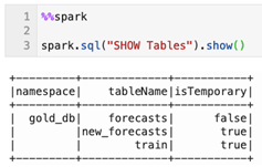
%%spark

db_name = "gold_db"
spark.sql("CREATE DATABASE IF NOT EXISTS " + db_name)

spark.sql("USE " + db_name)
%%spark spark.sql("""create table if not exists forecasts ( date date, store integer, item integer, sales float, sales_predicted float, sales_predicted_upper float, sales_predicted_lower float, training_date date ) using delta partitioned by (date)""") spark.sql("""merge into forecasts f using new_forecasts n on f.date = n.ds and f.store = n.store and f.item = n.item when matched then update set f.date = n.ds, f.store = n.store, f.item = n.item, f.sales = n.y, f.sales_predicted = n.yhat, f.sales_predicted_upper = n.yhat_upper, f.sales_predicted_lower = n.yhat_lower, f.training_date = n.training_date when not matched then insert (date, store, item, sales, sales_predicted, sales_predicted_upper, sales_predicted_lower, training_date) values (n.ds, n.store, n.item, n.y, n.yhat, n.yhat_upper, n.yhat_lower, n.training_date)""") - Now how good (or bad) is each forecast? Let’s apply the same techniques to evaluate each forecast. Using the pandas function technique, we can generate evaluation metrics for each store-item forecast.
%%spark # schema of expected result set eval_schema =StructType([ StructField('training_date', DateType()), StructField('store', IntegerType()), StructField('item', IntegerType()), StructField('mae', FloatType()), StructField('mse', FloatType()), StructField('rmse', FloatType()) ]) # define function to calculate metrics def evaluate_forecast( evaluation_pd: pd.DataFrame ) -> pd.DataFrame: # get store & item in incoming data set training_date = evaluation_pd['training_date'].iloc[0] store = evaluation_pd['store'].iloc[0] item = evaluation_pd['item'].iloc[0] # calculate evaluation metrics mae = mean_absolute_error( evaluation_pd['y'], evaluation_pd['yhat'] ) mse = mean_squared_error( evaluation_pd['y'], evaluation_pd['yhat'] ) rmse = sqrt( mse ) # assemble result set results = {'training_date':[training_date], 'store':[store], 'item':[item], 'mae':[mae], 'mse':[mse], 'rmse':[rmse]} return pd.DataFrame.from_dict( results ) # calculate metrics results = ( spark .table('new_forecasts') .filter('ds < \'2018-01-01\'') # limit evaluation to periods where we have historical data .select('training_date', 'store', 'item', 'y', 'yhat') .groupBy('training_date', 'store', 'item') .applyInPandas(evaluate_forecast, schema=eval_schema) ) - Once again, let’s persists evaluation metrics. We will likely want to report the metrics for each forecast, so we persist these to a queryable delta table.
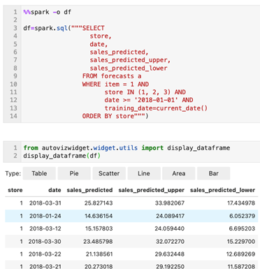
%%spark spark.sql("""create table if not exists forecast_evals ( store integer, item integer, mae float, mse float, rmse float, training_date date ) using delta partitioned by (training_date)""") spark.sql("""insert into forecast_evals select store, item, mae, mse, rmse, training_date from new_forecast_evals""") - We have now constructed a forecast for each store-item combination and generated basic evaluation metrics for each. To see this forecast data, we can issue a simple query (limited here to product one across stores one through three).
%%spark -o df

df=spark.sql("""SELECT
                  store,
                  date,
                  sales_predicted,
                  sales_predicted_upper,
                  sales_predicted_lower
                FROM forecasts a
                WHERE item = 1 AND
                      store IN (1, 2, 3) AND
                      date >= '2018-01-01' AND
                      training_date=current_date()
                ORDER BY store""")
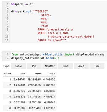
from autovizwidget.widget.utils import display_dataframe display_dataframe(df.head(6)) - Finally, let’s retrieve evaluation metrics.
%%spark -o df

df=spark.sql("""SELECT
                  store,
                  mae,
                  mse,
                  rmse
                FROM forecast_evals a
                WHERE item = 1 AND
                      training_date=current_date()
                ORDER BY store""")
from autovizwidget.widget.utils import display_dataframe display_dataframe(df.head(6))
We've now set up an OCI Data Science notebook and created an OCI Data Flow session to interactively run the Demand Forecasting application (PySpark) at scale.
To avoid incurring additional charges, delete or terminate all resources created to test this solution, and clean up the OCI Object Store buckets.
To get started with OCI Data Flow today, sign up for the Oracle Cloud Free Trial or sign into your existing account. Try Data Flow’s 15-minute no-installation-required tutorial to see just how easy Spark processing can be with Oracle Cloud Infrastructure.
