|
|
This chapter demonstrates various ways Oracle JRockit Mission Control can be used to monitor and manage application running on the Oracle JRockit JVM. It includes the following use cases:
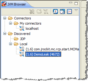
Marcus wants to monitor his application, DemoLeak which he’s running on an instance of the JRockit JVM, to ensure that he has tuned it to provide the best possible performance. To do this, he will run the JRockit Management Console concurrent with the application run. The Management Console will provide realtime information about memory, CPU usage, and other runtime metrics. The Management Console is a multi-tabbed interface, each tab allowing him to monitor and/or manage an aspect of a running application. Which tabs his version of the Management Console uses depends on which Java plug-ins he has installed with the console. When fully-implemented, the console will include eight tabs and one menu, which map to seven plug-ins.
To get started, Marcus launches the JRockit Mission Control Client from the command prompt, by entering:
jrockit\bin\jrmc
While the JRockit Mission Control Client is starting up, he launches the DemoLeak application. At the command prompt, he enters:
jrockit\bin\java DemoLeak
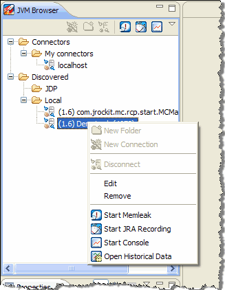
Next, he starts the Management Console with a local connection.
To launch the Management Console, Marcus does the following:
After a few moments, the Management Console appears in the right panel of the JRockit Mission Control Client. Note that in Marcus’s implementation of the JRockit Mission Control Client, he can see the following tabs:
One way to spot problems with application performance to is to see how it uses memory during runtime. To analyze how his application is using the memory available to it, Marcus will use the Memory Tab. This tab focuses on heap usage, memory usage, and garbage collection schemes. The information provided on this tab can greatly assist Marcus in determining whether he has configured the JRockit JVM to provide optimal application performance.
To analyze memory usage, Marcus does the following:
Next, he decides to see the duration for each garbage collection. Overly long garbage collection times are a common cause of poor application performance. To see the duration of the garbage collections, Marcus can plot this information on the Heap graph.
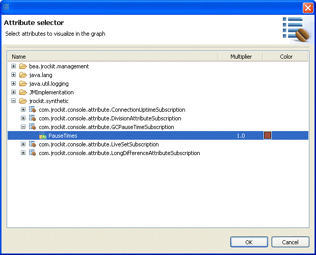
The graphs shown in the various tabs are all preconfigured with a few useful default attributes, but any numerical attribute from any MBean can be added. In addition to the standard MBeans in J2SE 5.0 and the JRockit JVM specific MBeans, JRockit Mission Control itself provides so called synthetic MBeans that derives attributes from multiple other attributes. One such attribute is the garbage collection times
| Note: | The attribute for garbage collection durations is called PauseTimes even though the Java application isn’t necessarily paused during the whole garbage collection. When a concurrent garbage collector is in use, the garbage collector runs concurrently with the Java application for the most part of the garbage collection duration. The misleading naming of the attribute is a known issue and will be fixed in upcoming releases. The correct name of the attribute would be Duration. |
To do this, Marcus does the following:
The Attribute Selector appears.
The new attribute should now be shown in the Heap graph. This synthetic attribute is a somewhat special in that it only shows values just before and after a garbage collection, causing the triangular-shaped plot, as shown in Figure 23-5. The value is shown in milliseconds.
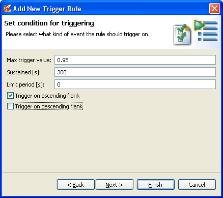
In his search for bottlenecks in the system, Marcus looks at the CPU load graph and notices that the CPU load for the JVM sometimes hits the roof. Marcus would like to know how often this happens for a longer period of time. Instead of staying and watching the CPU graph continuously he sets an alert trigger to alert him whenever the CPU load generated by the VM is high for a longer period of time.
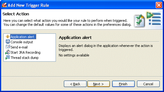
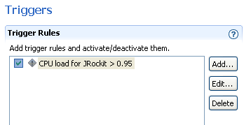
To set the alert, Marcus does the following:
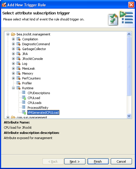
The Add New Trigger Rule wizard appears.
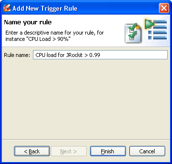
Since the CPU load value ranges from 0-1, Marcus sets the Max trigger value to 0.95. Marcus wants to be alerted when the CPU usage is high for at least five minutes and sets Sustained [s] to 300. He sets the Limit period [s] to 10 to prevent triggers less than 10 seconds apart.
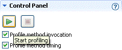
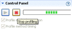
CPU load for JRockit > 0.95) and clicks Finish.Next, Marcus wants to see how many times and for how long some specific methods have run, a process called method profiling. JRockit Mission Control has two tools for profiling methods:
To profile methods by using the Method Profiler tab, Marcus does the following
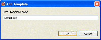
The Add Template dialog box appears.
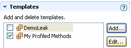
The dialog box closes and the new template is added to the list (Figure 23-12).
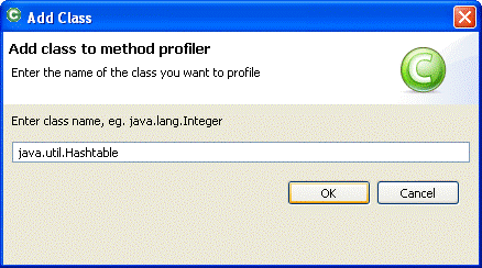
Add class to method profiler dialog box appears.
java.util.Hashtable, as shown in Figure 23-14java.util.Hashtable class, scrolls down and checks the boxes in front of the put(Object, Object) and remove(Object) methods, as shown inn Figure 23-15.Hashtable.put(Object, Object) grows slightly faster than the number of invocations of Hashtable.remove(Object).
Fiona is not happy with how the application DemoLeak is performing. She is particularly concerned about the way her application performs the longer it runs. For example, while the application works fine early in its run, after a while, it starts reporting the wrong results and throwing exceptions where it shouldn’t. She also notices that eventually, it hangs at roughly the same time every time she runs it. To assess what the problem is, Fiona decides to create a runtime analysis by use the JRockit Runtime Analyzer (JRA).
The JRA is an on-demand “flight recorder” that produces detailed recordings about the JVM and the application it is running. The recorded profile can later be analyzed off line, using the JRA Tool. Recorded data includes profiling of methods and locks, as well as garbage collection statistics, optimization decisions, and, in JRockit Mission Control 3.0, latency analysis.
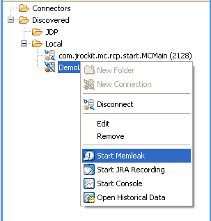
To start the diagnostics process, Fiona does the following:
Next, Fiona creates a JRA recording from a local connection. To do so, Fiona does the following:
| Note: | If Fiona sets a recording length that is too short, for example, less than 30 seconds, she will probably not get enough sample data for the recording to be meaningful. |
The JRA recording progress window appears. When the recording is finished, it loads in the JRA. Fiona will now look at the JRA Recording.
Next, Fiona will use the JRockit Mission Control Client to view the JRA recording. First, she opens the General tab by doing the following:
The JRA General tab for that recorded file now opens, allowing Fiona to view the data in the recording. The General tab contains information on the JVM, your system and your application. It is divided into the panels described in Table 23-2:
By looking at this tab, Fiona is able to verify which version of the JVM she was running. She can also see that large object were allocated at a rate, or “frequency”, of 22.153 MB per second while small objects were allocated at a significantly faster rate of 261.983 MB per second.
Next, Fiona will look at the Methods tab. The Method tab lists the top hot methods with their predecessors and successors during the recording. The Methods tab is divided into the following panels described in Table 23-3:
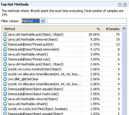
The method sampling in the JRockit JVM is based on CPU sampling. The Top Hot Methods section lists all methods sampled during the recording and sorts them with the most sampled method s first, as shown in Figure 23-18.
| Note: | If Fiona enabled native sampling during the recording, she would see symbols with a pound sign, such as jvm.dll#_qBitSetClear. These denote functions in native libraries such as the JVM itself or various operating system libraries. |
By looking at the list of top hot methods, Fiona sees that the three hottest methods are:
Starting with this information, Fiona has a good idea of where to start looking for possible areas of concern. Fiona knows that the hottest methods are those that are sampled most often. In some situations, the number of samplings in the hottest methods will dwarf those of the less-hot methods. Hot methods are a good indicator of performance problems, especially memory leaks, because the high amount of sampling affects how much time the JVM has been executing the specific method.
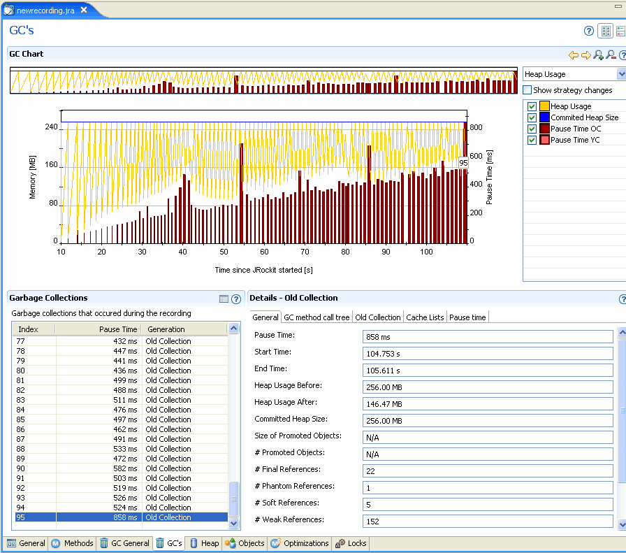
Next Fiona examines the GC’s tab (Figure 23-19) to better understand system behavior and garbage collection performance during runtime.
This tab is divided into the six panels described in Table 23-4
This graph shows heap usage compared to pause times and how that varies during the recording. When Fiona selects a specific area in the GC Events Overview, she only sees that section of the recording. She can change the graph content in the Heap Usage drop-down list (marked 6 in Figure 23-19) to get a graphical view of the references and finalizers after each old collection.
|
|
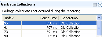
Looking at the data in the Garbage Collections panel (Figure 23-20), Fiona sees that the three longest garbage collection pause times are indexed 95 (856 ms), 41 (707 ms), and 73 (691 ms).
This data implied that, as processing continued on her application, garbage collections were taking longer. Fiona now has additional evidence to help diagnose what might be causing her application’s performance to deteriorate. She sees that garbage collection times are increasing, particularly later during runtime, and that the garbage collections are freeing less space on the heap. She can, with some confidence, predict that she is experiencing a memory leak.
| Note: | In this example, a memory leak is revealed to Fiona fairly quickly and she finds it because the evidence is obviously pointing in that direction. In most cases, a memory leak will reveal itself much more slowly and probably wouldn’t be obvious on the GC’s tab. Instead, a user would get better results by using the JRockit Memory Leak Detector, as described in Detecting a Memory Leak. |
Fiona can gain more insight into how garbage collection activity might be indicating a memory leak by looking at the GC General tab (Figure 23-21).
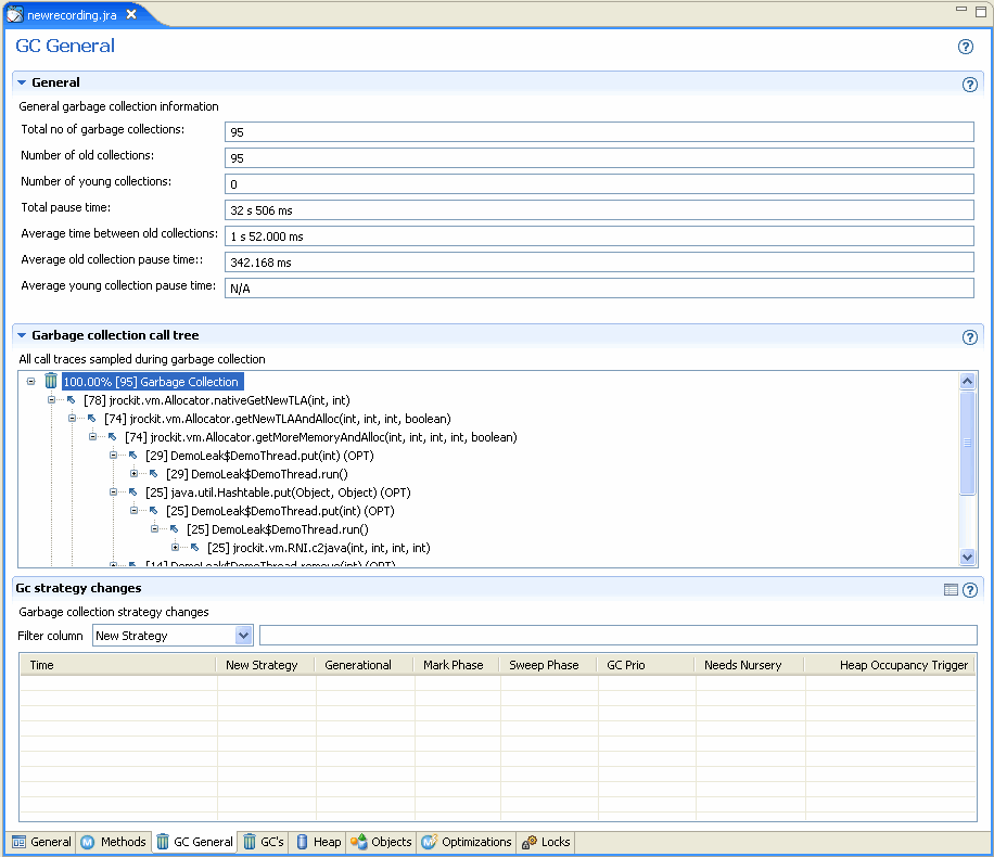
This tab is divided into three panels that provide information about the garbage collection at a glance. This tab is divided into the panels described in Table 23-5:
Fiona expands the stack tree down to user code and sees that many allocations are from the hashtable type, which indicates that this type is allocation intense. Reducing the allocation of this type would probably reduce the pressure on the memory management system.
Next, Fiona decides that it would be helpful to compare object statistics collected at the beginning of the recording to those collected after the recording. At the beginning and at the end of a recording session, snapshots are taken of the most common types and classes of object types that occupy the Java heap; that is, the types of which the total number of instances occupy the most memory. The results are shown on the Objects tab (Figure 23-22).
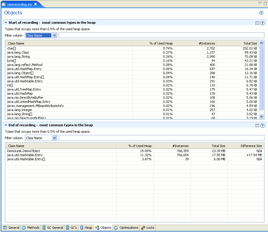
The Object Statistics tab is divided into the panels described in Table 23-6.
Fiona can again see that hashtable shows the most dramatic growth and is consuming the greatest amount of memory on the heap. This again is a strong indication of not only a memory leak but that said leak involves the hashtable object.
Fiona then checks the lock statistics for clues to performance bottlenecks involving locks. She opens the Locks tab (Figure 23-23) to investigate this information for both her application and the specific JRockit JVM instance.
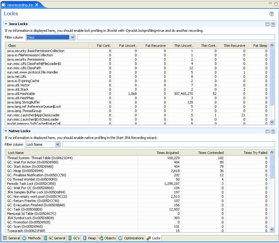
The Lock Profiling tab is divided into the panels defined in Table 23-7.
By looking at the Java Locks panel, Fiona can see immediately that the hashtable type has taken over 300 million uncontended locks, compared to a relative few for other objects. While this information does not point directly to a memory leak, it is indicative of poor performance.
Since the lock is mostly uncontended, Fiona could optimize her application by switching to an unsynchronized data structure such as hashmap and provide synchronization only for the few cases where contention may occur.
Since Fiona determined that a memory leak is causing her application to run poorly, she can take advantage of the JRockit Memory Leak Detector to confirm her suspicions and begin corrective action. A memory leak occurs when a program fails to release memory that is no longer needed. The term is actually a misnomer, since memory is not physically lost from the computer. Rather, memory is allocated to a program, and that program subsequently loses the ability to access it due to program logic flaws.
To start the memory leak detection process, Fiona does the following:
| Note: | This procedure assumes that the application was stopped after the JRA recording was completed. Had Fiona not stopped the application, she would be able to skip step 1 and step 2 |
java DemoLeak
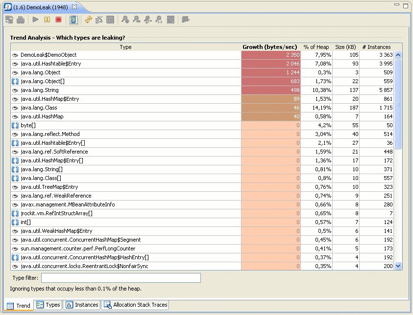
Fiona starts the analysis from the Trend tab (Figure 23-25), which should open when she launches the Memory Leak Detector.
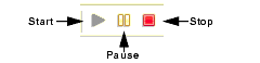
| Tip: | The trend analysis should be running by default. If it is not running, you can start it by clicking the start symbol among the trend analysis buttons (Figure 23-27). |
The trend analysis page shows Fiona the statistics on memory usage trends for the object types within the application. The JVM collects this data during garbage collections, which means that at least two garbage collections must be done before any trends are shown.

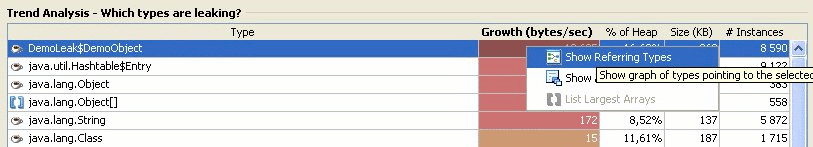
Fiona finds that a class named DemoObject shows the largest growth.
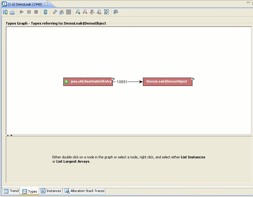
This opens the Types tab (Figure 23-29). Here Fiona can see that the DemoObjects are stored in hashtable entries.
Now Fiona can see that the DemoObjects are indeed stored in hashtable entries. The next step for Fiona is to find out more about the instances holding on to the hashtable entries containing these DemoObjects.
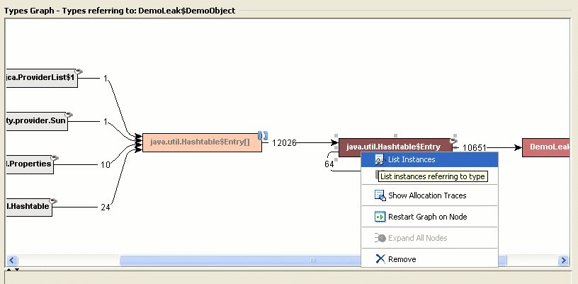
Not all hashtable entries in the application point to the same type of objects, so Fiona gets a popup that asks her to select the type of references she is interested in.
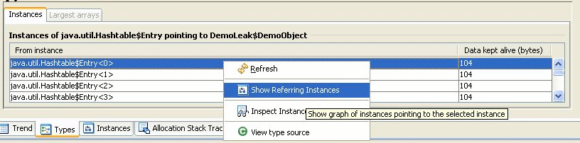
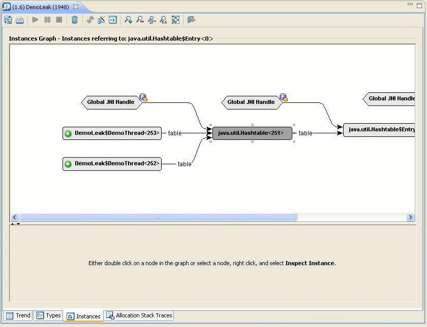
At the bottom of the Types tab Fiona gets a list of instances of java.util.Hashtable$Entry that refer to DemoObjects.
This opens the Instances tab, as seen in Figure 23-33.
Fiona finds that the DemoObject is stored in a hashtable, which is held by a DemoThread. This is the culprit causing the memory leak.
Judging from the evidence she collected using the Oracle JRockit Mission Control tools, Fiona was able to not only identify her system problem as a memory leak, but was able to locate exactly which object type was leaking the memory. The key to making the identification began with noting in her JRA recording the increasing length of garbage collections and the types upon which those lengthening garbage collections were occurring. She then ran the Memory Leak Detector to pinpoint which of the questionable types were actually the source of the leak. She was able to spot types that continued to increase in their number of instances and allocations, obviously holding on to memory so that it couldn’t be freed for allocating other objects. This, then identified the memory leak and where it was occurring.


|