Creating Worksheets and Content Panes

This chapter covers the following topics:

• Introduction
• Working with Lists
• Creating or Editing a Worksheet or Content Pane
• Configuring the Basics
• Selecting Series on a Worksheet
• Managing the Series Lists
• Specifying the Time Resolution and Time Span
• Specifying Aggregation Levels
• Using the Advanced Selection Options
• Changing the Overall Scale or Unit of Measure
• Filtering the Worksheet or Content Pane
• Managing the List of Members
• Applying Exception Filters
• Defining the View Layout
• Adding and Managing Worksheet Views
• Specifying the Worksheet Elements in a View
• Displaying an Embedded Worksheet
• Filtering a Worksheet View
• Sharing Worksheet and Content Panes
• Deleting Worksheet or Content Panes
• General Tips on Worksheet Design

Introduction

This chapter describes how to create and redefine worksheets and content panes.

To create or redefine worksheets and content panes, you use the worksheet editor, which is divided into multiple screens. This section provides a quick overview:

Area	Purpose	For details, see
Display	Specify basic information.	Configuring the Basics
Series	Select series to include.	Selecting Series on a Worksheet
Time	Specify time resolution of worksheet or content pane and span of time to consider.	Specifying the Time Resolution and Time Span
Aggregation Levels	Optionally specify aggregation levels to include.	Specifying Aggregation Levels
Filters	Optionally filter the selected combinations.	Filtering a Worksheet View
Exceptions	Optionally apply exception filters to further filter the combinations.	Applying Exception Filters
Layout Designer	Applicable only to worksheets. Define the layout of the worksheet and its views, including the layout of the worksheet tables, the location of each included series, and the graph format.	Defining the View Layout

Within the editor, you have the following options:

• To move to another page, either click a button on the left side of the page or click Previous or Next.

• To exit the worksheet editor and keep your changes, click OK.

• To exit the worksheet editor and discard all changes, click Cancel.

Working with Lists

As you create or edit worksheets and content panes, you will often use pages that present two lists of elements, where you specify your selections. To do so, you move elements from the left list to the right list. The left list always presents the available elements (such as the available series) and the right list always shows your selections.

You can move elements from one list to the other in many equivalent ways, summarized here:

• To move all elements from one list to the other, click one of the double arrow buttons, as appropriate.

• To move a single element from one list to the other, click the element and then click one of the single arrow buttons, as appropriate. Or double-click the element.

• To move several adjacent elements, click the first element, press Shift and click the last element. Then click one of the single arrow buttons, as appropriate.

• To move several elements that are not adjacent, press Ctrl and click each element you want. Then click one of the single arrow buttons, as appropriate.

Creating or Editing a Worksheet or Content Pane

To create a new worksheet or content pane

Click File > New. Or click the New button.

To edit an existing worksheet or content pane

1. Click File > Open. Or click the Open button.

2. Click a worksheet or content pane and click Open.

3. Click the Worksheet menu and select one of the menu items. Or click one of the worksheet buttons on the tool bar.

4. Save your changes to the worksheet definition: To save the new definition, click the Save button. Or click File > Save

   Note: In contrast, the Data > Update option saves the data and notes in the worksheet, not the worksheet definition.

   To save the worksheet with a new name, click the Save As button.

Configuring the Basics

To configure basic information for a worksheet or content pane

1. Click Worksheet > Display. Or click the Display button.

   The system displays a page where you specify the following basic information

   

   Name	The title to use in the My Worksheets module and in the window title.
   Description	Provides optional information to display in My Worksheets. This is especially useful in public worksheets for explaining the purpose of the worksheet to other users.
   Access	Select Private or Public. Private is for your use only. Public worksheets and content panes are available to all users in the group.
   Enable Extra Filters	This option adds an extra, user-controlled filter to the worksheet. If you select the Enable Extra Filters check box, that means that when you open the worksheet, you can prefilter the data before seeing the worksheet results; this is especially useful for users who use Demantra Anywhere. Normally when you specify aggregation levels to include in the worksheet, as described in "Specifying Aggregation Levels", all members of those levels are available in the worksheet. If you select the Enable Extra Filters check box, that means that when you run the worksheet, Demantra first prompts you to select the members to display for each level. This option has no effect on content panes.
   Cache Worksheet Data	Specifies whether Demantra should cache the data for this worksheet, for each user who works with it. If you cache a worksheet, it will run more quickly in general, but the cache will need to be refreshed periodically. Choose one of the following refresh options: Manual—users will have to manually refresh the cache. Automatic—Demantra will automatically refresh the cache, as specified by your implementors. In either case, Demantra automatically detects when a cache is out of date and behaves appropriately. Demantra also automatically refreshes the cache when you make certain structural changes to the worksheet.
   Open With Context	Specifies how this worksheet should be filtered when a user opens it via the Open or Open With menu options (on the right-click menu). Choose one of the following options: Selected Member (this will filter the worksheet to the object from which it was launched, aggregating across all combinations associated with that object) Selected Combination (this will filter the worksheet to the combination from which it was launched)

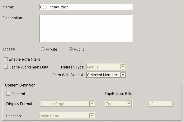
2. To display the content of this worksheet as a content pane in Collaborator Workbench, check Content and then complete the following fields:

   Display Format	Specifies the display format to use. Not all display formats may be possible, depending on the number of levels and series you include. Currently, Collaborator Workbench chooses the color to use for each series, when displaying series in the graph-type content panes.
   Location	Select Wide Pane or Narrow Pane to determine where the content pane will be displayed in Collaborator Workbench.
   Top/Bottom Filter	(Only for bar chart content panes.) Specifies how to filter the members or combinations for display in the bar chart (to save space, not all members are shown). Use the dropdown menu to specify whether the filter should apply to the top-ranked or to bottom-ranked members. In the input field, specify the number of members to be included. For Criteria Series, select the series that Demantra should use to rank the members. (This does not control the order in which they are displayed in the chart.) Note: If multiple items have identical values, all of them are displayed, and they collectively count as 1 towards the total. For example, suppose top values were 200, 150, 150, 100, and 50. If you specified Top/Bottom filter as three, you would see a total of four items: both the 150 items, in addition to the 200 and 100 items. This option does not affect the worksheet.

3. For worksheets only, to specify how the table should appear, see Defining the View Layout.

Selecting Series on a Worksheet

Every worksheet or content pane must include at least one series.

Note: If you use a settlement level in a worksheet or content pane, all series in the worksheet or content pane must refer to tables used by the settlement hierarchy.

To specify the series on a worksheet or content pane

1. Click Worksheet > Series. Or click the Series button.

   The system displays the Available Series and Selected Series lists. Each list is a collapsible list of series groups and the series in them.

   

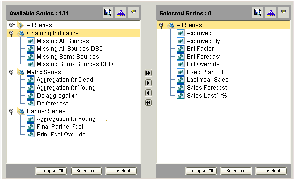
2. Move all series that you want into the Selected Series list. To do so, either double-click each series or drag and drop it. You can also move an entire series group from one list to the other in the same way.

3. Remove any series from the Selected Series list that you do not want to include.

   Note: You cannot remove a series if it is used as the Criteria Series for bar chart content.

   To change the order in which the series are displayed, see Defining the View Layout.

   See Managing the Series Lists.

Managing the Series Lists

You may have a very large number of series, and it can be useful to sort and filter these lists so that you can readily find what you need. The system also provides a search mechanism.

Note: This section applies only to the series page of the worksheet editor (Worksheet > Series).

To sort a list of series

1. Click the Sort button.

   The Sort dialog box is displayed.

2. Drag the list name from the Available Columns to the Sort Columns. Or double-click the list name in the Available Columns list.

3. Click OK.

To filter a list of series

1. Click the Filter button.

   The Filter page appears.

2. Click Add.

3. Click the arrow to the right of the operator box and select an operator from the dropdown list.

4. In the number box, enter the value by which to filter the list.

5. (Optional) You can filter further by using the AND relationship.

6. Click OK.

To find a series

1. Click the Find button.

   The Find dialog box appears.

2. In the Find where box, select the name of the list to search.

3. In the Find what box, type name of the series.

4. Select Up, Down or All to determine the direction of the search.

5. (Optional) Select one or more of the check boxes:

   • Whole Word: Search for the exact match of a word.

   • Match Case: Search for the exact match of a word (case sensitive).

6. Click Find Next to begin (or continue) searching.

Specifying the Time Resolution and Time Span

Each worksheet or content pane selects data for a specified span of time and optionally aggregates it in time. You use the Time dialog box to specify the time resolution and span of time of the results.

To specify time criteria

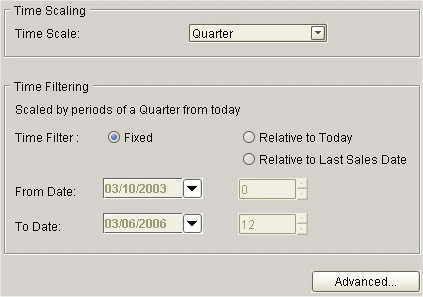
1. Click Worksheet > Time. Or click the Time button.

2. In the Time Scale box, specify the time resolution. The data in the worksheet or content pane is aggregated to this time resolution. That is, this option specifies the period of time that each data point in the line graph represents.

3. In the Time Filter box, specify the time period to which the worksheet or content pane applies:

   • Fixed if you always want to show a specific time range, regardless of the current date.

   • Relative to Today if you always want to show a time range relative to today.

   • Relative to Last Sales Date if you always want to show a time range relative to the last sales date in the loaded data.

4. In the From Date and To Date boxes, enter values depending on the time filter you have chosen, as follows:

   Time Filter	Box	Action
   Relative	From Date / To Date	Specify periods in both From and To with the current (computer) date as the reference point. For example: If the Time Scale is Month, and you want to see results starting from six months before today, enter -6 in From Date.
   Fixed	From Date	Enter a specific date as a starting point of the results. To enter a date, click the calendar button and select a date.
   Fixed	To Date	Specify the number of periods you want to include, starting from the From date.

5. To control how dates are displayed, click the Advanced button, which brings up the following dialog box:

   

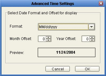
6. In the Format dropdown list, select a display format.

   For example, to add one month to each displayed date, specify 1 for Month Offset.

   The Preview field shows what the first time bucket would look like with this format and offset.

7. To offset the displayed dates, optionally specify values for Month Offset or Year Offset.

8. Click OK.

   Note: If you change the time scale, the worksheet or content pane might not show exactly the same aggregate numbers, because the cutoff dates would not necessarily be the same. For example, suppose your worksheet is weekly and displays 48 weeks of data. Then supposed you change the worksheet to display quarterly data. A quarter is 13 weeks, and the original span (48 weeks) is not an integer multiple of 13. So the worksheet selects a different amount of data and shows different overall results.

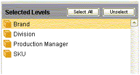
Specifying Aggregation Levels

A worksheet or content pane usually includes aggregation levels. When you use the worksheet or content pane, you can examine data for the item-location combinations associated with those levels.

• If you do not specify any aggregation levels, the data is completely aggregated across all items and locations.

• If you use a settlement level, you cannot use levels from any other hierarchy.

To specify the aggregation levels in a worksheet or content pane

1. Click Worksheet > Aggregation Levels. Or click the Levels button.

   The system displays the Available Levels and Selected Levels lists.

2. Move all aggregation levels that you want into the Selected Levels list, using any of the techniques in "Working with Lists".

3. Remove any unwanted levels from the Selected Levels list.

   

   For a worksheet, the selected levels will now be used on all views of this worksheet, unless you configure the views otherwise. The layout of the worksheet view controls the order in which the levels are used; see Defining the View Layout.

   See also

   • Using the Advanced Selection Options

   • Changing the Overall Scale or Unit of Measure

Using the Advanced Selection Options

By default, if a worksheet or content pane includes a promotion level, the worksheet or content pane includes all the following types of combinations:

• Combinations that have both sales data and promotions

• Combinations that have sales data, but no promotions

• Combinations that have promotions, but no sales data

The worksheet or content pane displays placeholders for combinations that do not have promotions. For example:

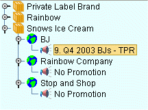
For a worksheet, if you move the promotion level to the worksheet axis (see Defining the View Layout), the table will display a similar placeholder.

You can exclude some of these combinations. For example, you might want a worksheet to include only the combinations that have both sales and promotions, as follows:

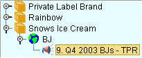
To exclude combinations with partial data

1. Click Worksheet > Aggregation Levels. Or click the Levels button.

2. Include at least two levels, one of which should be a promotional level.

   When you do so, the screen displays an Advanced button in the lower right.

   

3. Click Advanced.

   Oracle displays a dialog box with additional options.

   

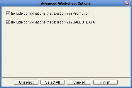
   Include combinations that exist only in Promotion	This option selects combinations that have associated promotions, even if they do not have sales data.
   Include combinations that exist only in SALES_DATA	This option selects combinations that have sales data, even if they do not have any associated promotions.

4. To exclude the combinations you do not want to see, click the check boxes as needed.

   See Specifying Aggregation Levels.

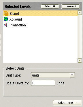
Changing the Overall Scale or Unit of Measure

In addition to levels, series, and filtering, a worksheet or content pane has the following characteristics:

• A single unit of measure. Typically, most series refer to this unit of measure, but there are exceptions such as percentage values. You can switch the unit of measure, and the displayed values are changed accordingly. The units in your system depend upon your implementation but probably include unit count and dollars.

  For monetary units, you can also switch to a different index (such as the Consumer Price Index or CPI) or exchange rate, and the worksheet or content pane automatically multiplies all values accordingly.

• An overall scale. The default value is 1. If the displayed values are all large, it can be useful to re-scale the numbers, for example, to display in amounts of 1000 or 1000000.

You can change either or both of these. When you make this change, the displayed values for most or all of the series in the worksheet or content pane are changed.

Note: This change affects only the series that are scaled. Not all series are scaled. For example, a series defined as a percentage is probably not scaled.

To change the overall scaling factor

1. Click Worksheet > Aggregation Levels. Or click the Levels button.

   The Levels page includes a section where you specify the overall scale of the worksheet or content pane, as well as its units of measure.

   

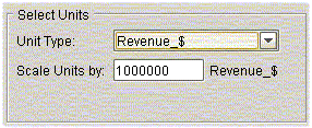
2. In the Scale Units by box, specify the factor by which all numbers are to be divided (for display purposes).

   For example, if you specify a factor of 1000, the displayed data will divided by 1000. So the number 96,000 will be displayed as 96. The vertical axis of the graph is updated to show the factor in parentheses. For example, if the vertical axis was formerly labeled "units", it will be updated to say "units (1000)" instead.

To change the unit of measure

1. Click Worksheet > Aggregation Levels. Or click the Levels button on the toolbar.

2. In the Unit Type box, select the unit of measure to display in the worksheet or content pane results.

   For example, our items are bottles, and suppose that a case that contains six bottles. If you display the worksheet or content pane with cases instead, the system will display the number of bottles divided by six.

3. If the Index box is displayed, choose an index from the dropdown list.

   

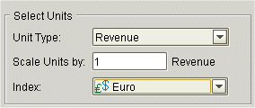
   The Index menu lists all the time-dependent indexes and exchange rates that are associated with this unit. Each index or exchange rate is a time-varying factor that the worksheet or content pane can use. When you select an index, the worksheet or content pane will automatically multiply all monetary series by the factor for each date. For example, if you choose Consumer Price Index (CPI) as the index, the system will calculate all monetary quantities with relation to the CPI.

   Note: These indexes and exchange rates are generally imported from other systems. The set available to you depends upon your implementation.

   See Specifying Aggregation Levels.

Filtering the Worksheet or Content Pane

Filters control the combinations that you are able to see. Filtering can have multiple sources:

• A given worksheet or content pane may be filtered. For example, worksheet X might show only Brand X, which means that the worksheet would show only combinations related to Brand X.

• Your user ID may be filtered. For example, if you are an account manager, your user ID might give you access only to your accounts. At any level, you would not be able to see combinations associated with other accounts.

• The data that you share with other users (called the component) might also be filtered. Components divide the data for different sets of users.

Demantra automatically combines all the filters. In the preceding example, if the component is not filtered, if you use worksheet X, you can see only data for Brand X at your accounts.

In contrast to an exception filter ("Applying Exception Filters"), this type of filter is static and behaves the same no matter how the data changes.

To apply a filter to a worksheet or content pane

1. Click Worksheet > Filters. Or click the Filters button.

   The system displays the Available Filter Levels and Selected Filter Levels lists.

2. Find the aggregation level at which you want to filter data and move it from the Available Filter Levels list into the Selected Filter Levels list, using any of the techniques in "Working with Lists".

   Note: This level does not have to be the same as any of the aggregation levels you display in the worksheet or content pane. In fact, typically you filter using a different level than you use to display.

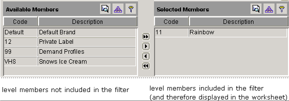
3. In the Available Members list, find a member that you want to include and move it into the Selected Members list, using any of the techniques in "Working with Lists.".

   At this stage, the worksheet or content pane includes only data for this member. (Before you applied a filter at this level, the worksheet or content pane could theoretically include any member of this level.)

4. Continue to move members from the Available Members list into the Selected Members list, until the latter list includes all the members you want.

   

To filter data further

Once you have applied a filter as described previously, the worksheet or content pane contains only those combinations that are associated with the members you specified. You can further filter the data in exactly the same way.

See Applying Exception Filters.

Managing the List of Members

Depending on how your system has been configured, it might contain a very large number of members. If so, you might want to sort or filter the list or search it. For information, see Managing the Series Lists.

Applying Exception Filters

If you attach an exception filter, Demantra checks the values of the data and displays only the combinations that meet the exception criteria. In contrast to an explicit filter, Filtering the Worksheet or Content Pane, this type of filter is dynamic and can behave differently as the data changes.

Specifically, you define an exception condition that consists of a series, a comparison operator, and a value, for example:

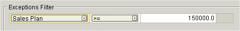
When you open the worksheet, Demantra checks each combination in the worksheet. For each combination, if the condition is met for any time in the worksheet date range, Demantra displays that combination. For example, the worksheet shows combinations that have Sales Plan values greater than or equal to 150000, within the time range included in the worksheet.

If the condition is not met at any time for any of the worksheet combinations, Demantra shows the worksheet as empty. That is, if all values in the Sales series are less than 15000 for all combinations, the worksheet comes up empty.

Note: If the worksheet includes a promotion level or a promotion series, the behavior is slightly different. In this case, the Members Browser or dropdown list does initially show all combinations. When you click display a combination to display it, the worksheet then checks for exceptions.

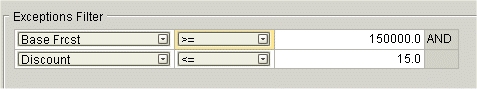
You can apply multiple exceptions to a worksheet. When you apply multiple exceptions, you can relate them to each other via logical AND or logical OR relationships. For example:

To apply an exception filter

1. Click Worksheet > Exceptions. Or click the Exceptions button.

   The Exceptions Filter page appears.

2. Click Add.

3. In the first box in the new row, select a series from the dropdown list.

   Note: Typically only some series are available for exceptions. If you do not see a series you need, contact your Demantra administrator or your implementors.

4. In the second box, select an operator from the dropdown list.

5. In the third box, type or choose a value.

   

   • For a numeric series, type a number.

   • For a dropdown series, choose one of the allowed values of this series.

   • For a string-type series, type any string. You can use the percent character (%) as a wildcard.

   • For a date-type series, type a date or use the calendar control to choose a date.

6. (Optional) You can apply additional exceptions. Select the AND or the OR radio button to specify the relationship between the exceptions.

   

To delete an exception filter

1. Click the exception and then click Delete.

   See

   • Filtering the Worksheet or Content Pane.

Defining the View Layout

This section applies only to worksheets, not to content panes.

To define the layout of a current view

1. Click Worksheet > Layout Designer. Or click the Layout Designer button.

   The system displays a page where you specify the layout. This page displays the following areas:

   

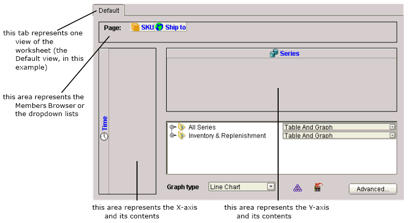
   In addition, this screen displays the following icons:

   • An icon for each aggregation level that you have included in the worksheet. By default, these levels are included in the Members Browser or selector lists.

   • An icon that represents the time axis. By default, time is shown on the x-axis.

   • An icon that represents the series data. Series are shown on the y-axis.

2. To change the worksheet layout, drag the level or time axis icons to the appropriate areas. You cannot move the series icon.

3. To specify the type of graph to use, select a graph type from the Graph Type dropdown list.

4. To specify how to display series in this view:

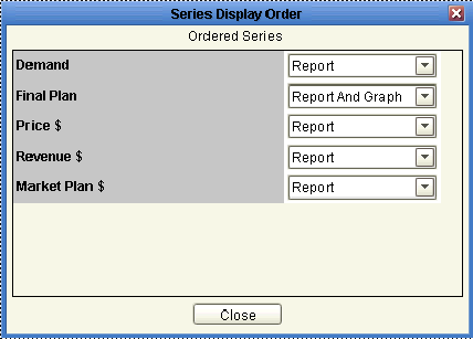
   1. Click the Sort button.

      The Layout Designer displays a page that shows the order in which this view currently displays the series.

      

   2. To hide a series in this view, click the None option in the dropdown list to the right of the series name.

   3. Otherwise, to specify where to display the data for a series, select one of the following options: Table, Graph, Table and Graph.

   4. To move a series up or down in this list, click the series name and drag it up or down.

   5. When you are done, click Close.

5. Click Save.

6. Rerun the worksheet to see your changes. To do so, click Data > Rerun.

To specify a cross-tab layout

1. Drag one or more level icons from the Page Item area to x-axis or y-axis areas.

To specify which levels to use in a worksheet view

By default, all levels you include in a worksheet are used on all views of the worksheet. Within a multi-view worksheet, you often hide some of the levels in some views, so that each view is aggregated differently.

1. Right-click within the Page area of the Layout Designer.

   The system displays a menu like the following:

   

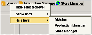
2. Click Hide level and then click the name of the level to hide.

   When you hide a level, the worksheet automatically aggregates data across members of that level.

   Note: Do not use this option to hide the time axis.

To revert to the default layout of a worksheet view

1. Click Worksheet > Layout Designer. Or click the Layout Designer button.

2. Click the tab corresponding to the worksheet view you want to reset.

3. Click the Reset button.

   In the default layout, all selected levels are visible and are on the X axis. Also, all series are displayed in the graph and table according to their default definitions.

   See

   • Specifying the Worksheet Elements in a View

   • Displaying an Embedded Worksheet

   • Filtering a Worksheet View

Adding and Managing Worksheet Views

This section applies only to worksheets, not to content panes.

A worksheet can include multiple views, each of which can have a different set of series and a different layout.

To add a worksheet view

1. Within the Layout Designer, click the Add Worksheet View button.

2. In the popup dialog box, type the name of the new view.

3. Click OK.

To control synchronization between the views

The views of a worksheet may or may not be synchronized with each other. If they are synchronized, when you edit in one view, that change automatically appears in the other views. Because this can affect performance, sometimes it is best to switch off this synchronization.

Within the Layout Designer, click one of the following buttons, whichever is currently displayed:

• Do not force synchronization between views

• Synchronize data between views

To rename a worksheet view

1. Within the Layout Designer, click the Rename Worksheet View button.

2. In the popup dialog box, type the new name of the view.

3. Click OK.

To enable or disable a worksheet view

1. Within the Layout Designer, click the Hide/Display button.

2. The Layout Designer displays a popup list of all the views associated with this worksheet. A check mark is displayed next to each view that can currently be displayed.

   

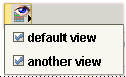
3. For the view interest, select the check box next to the name of the view.

4. Click elsewhere on the screen to close the list of views.

To delete a worksheet view

Within the Layout Designer, do one of the following:

• Click the tab that corresponds to the worksheet view. Then click the Delete Worksheet View button.

• Click the Delete All Worksheet View button. Then, at the prompt, click Yes.

See

• Defining the View Layout

• Specifying the Worksheet Elements in a View

• Displaying an Embedded Worksheet

• Filtering a Worksheet View

Specifying the Worksheet Elements in a View

This section applies only to worksheets, not to content panes.

For each worksheet view, you can specify which of the basic worksheet elements are included: the table, the graph, and so on.

To specify the elements to include in a worksheet view

1. Click Worksheet > Layout Designer. Or click the Layout Designer button.

2. Click the tab corresponding to the worksheet view you want to modify.

3. Click Advanced... in the lower right.

   Demantra displays the following screen:

   

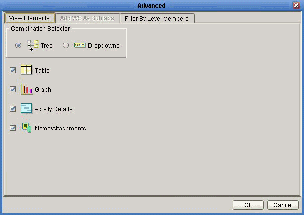
4. For Combination Selector, click either Tree (to display a Members Browser) or Dropdowns (to display dropdown menus instead).

5. Select the check box next to each element you want to include in this view of the worksheet.

6. Click OK.

Displaying an Embedded Worksheet

This section applies only to worksheets, not to content panes.

You can display embedded worksheets on subtabs within a view. An embedded worksheet can be at a higher aggregation level than the rest of the worksheet, and the worksheet itself remains editable in general.

Note: The choice of worksheets you see depends on the level-worksheet associations that are controlled within the Business Modeler.

To display an embedded worksheet as a subtab within a view

1. Click Worksheet > Layout Designer. Or click the Layout Designer button.

2. Click the tab corresponding to the worksheet view to which you want to add the sub tab.

3. Click Advanced... in the lower right.

   • Demantra displays the Advanced screen.

4. Click the Add WS As Subtabs tab.

   • Demantra displays a screen like the following:

     

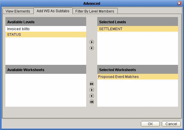
     Depending on the level that you select, the bottom part of the screen shows different worksheets that you can add as a subtab to this worksheet view.

5. For Selected Levels, select the level that is associated with the worksheet you want. In general, a worksheet is associated with the levels where it makes sense to use it; this is controlled by your system configuration. You can choose any of the levels that are used in this worksheet.

6. For Selected Worksheets, select the worksheets that you want to display as sub tabs within this worksheet view.

7. Click OK.

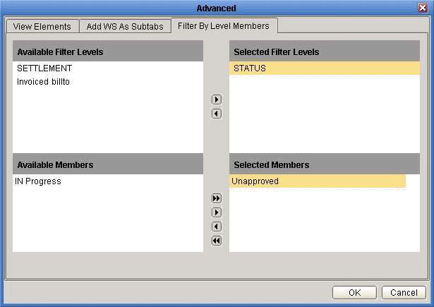
Filtering a Worksheet View

This section applies only to worksheets, not to content panes.

For each worksheet view, you can filter the view to show a subset of the data in the worksheet.

To filter a worksheet view

1. Click Worksheet > Layout Designer. Or click the Layout Designer button.

2. Click the tab corresponding to the worksheet view you want to filter.

3. Click Advanced... in the lower right.

   • Demantra displays the Advanced screen.

4. Click the Filter By Level Members tab.

   • Demantra displays a screen like the following:

     

5. For Selected Filter Levels, select the level by which you want to filter this worksheet view. You can choose any of the levels that are used in this worksheet.

6. For Selected Members, select the level members whose data should be displayed in this worksheet view.

7. Click OK.

Sharing Worksheet and Content Panes

In general, any worksheet or content pane is one of the following:

• Private—available only to you

• Public—available to other users as well. (If you are using Collaborator Workbench, this means the worksheet or content pane is available to others users within the collaborative group.)

In either case, the original creator owns it and only that person can change it.

When you do share worksheet and content panes, however, you should consider data security. Demantra automatically prevents any user from seeing data for which he or she does not have permissions. If you build a worksheet or content pane with data that other users do not have permissions to view, then those users will see an empty worksheet or content pane. Similarly, if a user has partial permissions for the data, then the worksheet or content pane will open with only those results that are permitted.

See Configuring the Basics.

Deleting Worksheet or Content Panes

You can delete a worksheet or content pane if you are its owner.

To delete a worksheet or content pane

1. Open the worksheet or content pane.

2. Click File > Delete. Or click the Delete button.

   • Demantra prompts you to confirm the deletion.

3. Click Yes or No.

General Tips on Worksheet Design

This section applies mostly to worksheets, not to content panes.

• For performance reasons, don't select too much data to view, unless there is no other choice.

• If you receive a message saying "out of memory," try the following techniques to reduce the amount of memory that your worksheet selects:

  • Remove series if possible

  • Reduce the span of time

  • Apply filters

• If you do need to select a large amount of data, use the levels to your advantage. Specifically, use the levels in the Members Browser or selector lists rather than moving them to a worksheet axis. If levels are in the Members Browser or selector lists, each combination in the worksheet is relatively smaller and will load more quickly.

• If you do not plan on working with the Activity Browser, you can switch off the Auto Sync option on the toolbar, and you can also hide the Activity Browser and Gantt chart.

• Remember that you can filter the worksheet by any level, including levels that are not shown in the worksheet. For example, you might want to see data at the region level, but exclude any data that does not apply to the Acme territory. To do this, you would filter the worksheet to include only the Acme member of the Territory level, but you would select data at the Region level.

• A multi-view worksheet is useful in following cases:

  • If you need to edit data at one aggregation level and see easily how that affects higher aggregation levels.

  • If you need to display a large number of series without having to scroll to see each one.