Transfer Pricing Option Costs
This chapter describes how Oracle Transfer Pricing goes about calculating option costs. The chapter begins with an introduction to option costs and subsequently describes option cost theory and the calculation architecture.
This chapter covers the following topics:
- Overview of Transfer Pricing Option Costs
- Understanding the Option Cost Calculation Architecture
- Option Cost Theory
- Option Cost Model Usage Hints
Overview of Transfer Pricing Option Costs
The purpose of option cost calculations is to quantify the cost of optionality, in terms of a spread over the transfer rate, for a single instrument. The cash flows of an instrument with an optionality feature change under different interest rate environments and thus should be priced accordingly.
Consider a mortgage that may be prepaid by the borrower at any time without penalty. Here the lender has, in effect, granted the borrower an option to buy back the mortgage at par, even if interest rates have fallen in value. Thus, this option has a cost to the lender and should be priced accordingly.
Another example of an instrument with an optionality feature is an adjustable rate loan issued with rate caps (floors) which limit its maximum (minimum) periodic cash flows. These caps and floors constitute options.
When banks give such options to their borrowers, they raise the bank's cost of funding the loan and affect the underlying profit. Consequently, banks need to use the calculated cost of options given to their borrowers in conjunction with the transfer rate to analyze profitability.
Oracle Transfer Pricing uses the Monte Carlo technique to calculate the option cost. The application calculates and outputs two spreads, and the option cost is calculated indirectly as a difference between these two spreads.
-
Static spread
-
Option-adjusted spread (OAS)
The option cost is derived as follows:
option cost = static spread - OAS
The static spread is equal to the margin, and the OAS to the risk-adjusted margin of an instrument. Therefore, the option cost quantifies the loss or gain due to risk.
You can calculate option costs using the Transfer Pricing Process rule. See: Transfer Pricing Process Rules, Oracle Transfer Pricing User Guide.
Understanding the Option Cost Calculation Architecture
This description of the option cost calculation architecture makes use of an example and assumes:
-
The instrument, taken in the example, pays K cash flows, each occurring at the end of the month.
-
Each month has the same duration in number of years, such as 1/12.
-
The discount factor calculation does not use the approximation for small option adjusted spread.
Related Topics
Overview of Transfer Pricing Option Cost
Defining the Static and Option-Adjusted Spreads
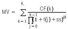
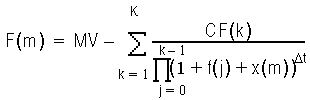
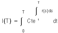
You can define neither the static nor the option-adjusted spread directly, as they are solutions of two different equations. Therefore, the system solves a simplified version of the equations. The static spread is the value ss that solves the following equation:
Here:
-
MV = market, book, or par value of the instrument
-
CF(k) = cash flow occurring at the end of month k along the forward rate scenario
-
f(j) = forward rate for month j
-
Delta T = length (in years) of the compounding period; hard-coded to a month, such as 1/12
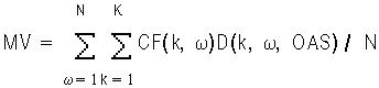
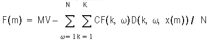
In the Monte Carlo methodology, the option-adjusted spread is the value OAS that solves the following equation:
Here:
-
N = total number of Monte Carlo scenarios
-
CF(k, w) = cash flow occurring at the end of month k along scenario w
-
D (k, w, OAS) = stochastic discount factor at the end of month k along scenario w for a particular OAS
Note: Cash flows are calculated until maturity even if the instrument is adjustable. Otherwise the calculations would not catch the cost of caps or floors.
In real calculations, the formula for the stochastic discount factor is simplified.
Related Topics
Understanding Option Cost Calculation Architecture
Option Cost Calculations Example
In this example, the transfer pricing yield curve is the Treasury curve. It is flat at 5%, which means that the forward rate is equal to 1%. This example uses only two Monte Carlo scenarios:
-
Up scenario: One-year rate one year from now equal to 6%.
-
Down scenario: One-year rate one year from now equal to 4%.
The average of these two stochastic rates is equal to 5%.
The instrument record is two year adjustable, paying yearly, with simple amortization. Its rate is Treasury rate plus 2%, with a cap at 7.5%. Par value and market value are equal to $1.
For simplicity, this example assumes that the compounding period used for discounting is equal to a year, for example:
Delta t = 1
The static spread is the solution of the following equation:
1 = [0.07 / (1 + 0.05 + SS) ] + [(1 + 0.07) / (1 + 0.05 + SS)2]
The static spread is supposed to be equal to the margin. In this example:
static spread = coupon rate - forward rate =7%-5%=2%
Substituting this value (2% or .02) in the right side of the above equation yields:
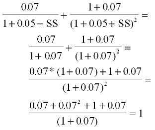
This is equal to par, which proves that the static spread is equal to the margin.
The OAS is the solution of the following equation:
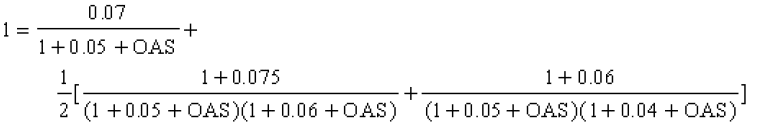
By trial and error you get a value of 1.88%.
To summarize:
option cost = static spread - OAS = 2%-1.88% = 12 basis points
Related Topics
Understanding Option Cost Calculation Architecture
Option Cost Calculations Process Flow
The following graphic represents the option cost calculations process flow.
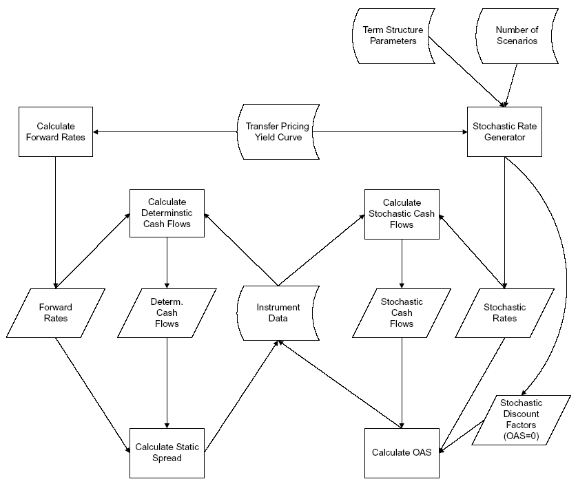
This exposition focuses only on the following steps:
-
Calculating forward rates
-
Calculating static spread
-
Calculating OAS
Related Topics
Understanding Option Cost Calculation Architecture
Calculating Forward Rates
The cubic spline interpolation routine first calculates smoothed, continuously compounded zero-coupon yields Y(j) with maturity equal to the end of month j. The formula for the one-month annually compounded forward rate spanning month j + 1 is:
fj = exp [ (Yj) (j + 1) - Y(j) j ] -1
Related Topics
Option Cost Calculations Process Flow
Calculating Static Spread
You can calculate the static spread using the Newton-Raphson algorithm. If Newton-Raphson algorithm does not converge, which can happen if cash flows alternate in sign, you can revert to a brute search algorithm. However, this algorithm is much slower.
You can control the convergence speed of the algorithm by adjusting the value of the variable OptionCostSpeedFactor. This variable is defined through a profile option, Option Cost Speed Factor.
The default value is equal to one. A lower speed factor provides more accurate results. In all experiments, a speed factor equal to one results in a maximum error (on the static spread and OAS), which is lower than half a basis point.
To recap the Newton-Raphson algorithm, let x be the static spread. At each iteration m, the function F(m) is defined by the following equation:
The algorithm is:
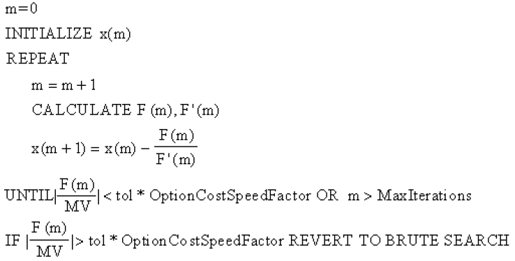
For performance reasons, the code utilizes a more complicated algorithm, albeit similar in spirit. This is the reason why the specific values for tol and MaxIterations, or details on the brute search are mentioned above.
Related Topics
Option Cost Calculations Process Flow
Calculating OAS
For fixed rate instruments, such as instruments having the same deterministic cash flows as the stochastic cash flows, the OAS is by definition equal to the static spread. This statement is true in the case of continuous compounding. For discrete compounding this approximation has a negligible impact on the accuracy of the results.
The OAS is also calculated with an optimized version of Newton-Raphson algorithm. See: Calculating Static Spread.
Note: While calculating OAS, the following substitution is made in the Newton-Raphson method: OAS = x(m)
Related Topics
Option Cost Calculations Process Flow
Option Cost Theory
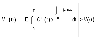
According to the option cost theory, when you select the market value of an instrument to equate the discounted stream of cash flows, the static spread is equal to margin and the OAS to the risk-adjusted margin of the instrument.
This exposition of option cost theory assumes that you have good knowledge of no arbitrage theory, and requires you to note these assumptions and definitions:
-
To acquire the instrument, the bank pays an initial amount V(0), the current market value.
-
The risk-free rate is denoted by r(t).
-
The instrument receives a cash flow rate equal to C(t), with
0 < = t < = T < = Maturity
-
The bank reinvests the cash flows in a money market account which, with the instrument, comprises the portfolio.
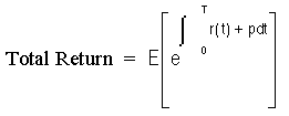
-
The total return on a portfolio is equal to the expected future value divided by the initial value of the investment.
-
The margin p on a portfolio is the difference between the rate of return (used to calculate the total return) and the risk free rate r.
-
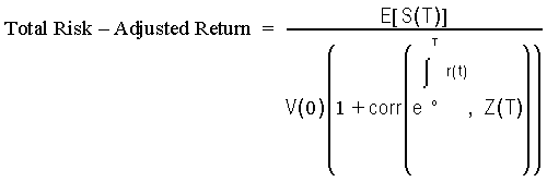
The risk-adjusted expected future value of a portfolio is equal to its expected future value after hedging all diversifiable risks.
-
The total risk-adjusted return of a portfolio is equal to the risk-adjusted expected future value divided by the initial value of the investment.
-
The risk-adjusted margin m of a portfolio is the difference between the risk-adjusted rate of return (used to calculate the total risk-adjusted return) and the risk-free rate r.
More precisely,
Related Topics
Overview of Transfer Pricing Option Cost
Equivalence of the Option Adjusted Spread and Risk-Adjusted Margin
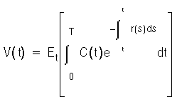
In a no-arbitrage economy with complete markets, the market value at time t of an instrument with cash flow rate C(t)is given by:
If expectation is taken with respect to the risk-neutral measure, the expected change in value is given by:
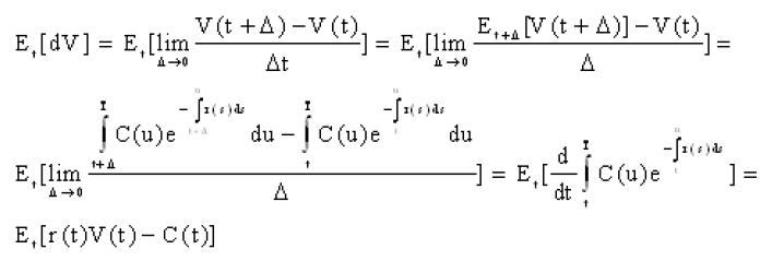
The variation in value is, therefore, equal to the expected value of the change dV plus the change in value of a martingale M in the risk-neutral measure:
dV(t) = Et[dV] + dM = rVdt - Cdt + dM
If I is the market value of the money market account in which cash flows are reinvested then:
Note that unlike V, this is a process of finite variation. By Ito's lemma:
dl = rIdt + Cdt
Let Sbe the market value of a portfolio composed of the instrument plus the money market account. We have:
dS = dV + dI = rSdt + dM
S(0) = V(0)
In other words, the portfolio, and not the instrument, earns the risk-free rate of return. An alternate representation of this process is:
dS/S = rdt + dN
Here N is another martingale in the risk-neutral measure. The expected value of the portfolio is then:
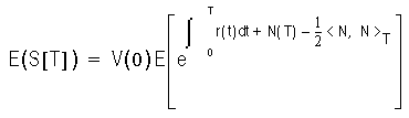
Here, <N, N> is the quadratic variation of N. This is equivalent to:

To define the martingale:
Z = eN-(1/2)<N,N>
This represents the relative risk of the portfolio with respect to the standard money market account, that is, the account where only an initial investment of V(0) is made. Then
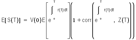
In other words, the expected future value of the portfolio is equal to the expected future value of the money market account adjusted by the correlation between the standard money market account and the relative risk. Assuming complete and efficient markets, banks can fully hedge their balance sheet against this relative risk, which should be neglected to calculate the contribution of a particular portfolio to the profitability of the balance sheet. Therefore:
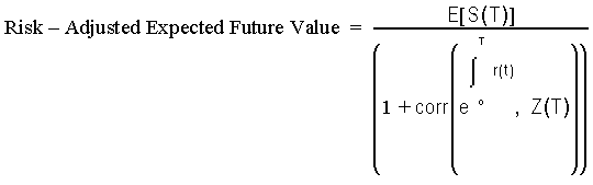
In this example, the risk-adjusted rate of return of the bank on its portfolio is equal to the risk-free rate of return.
Now suppose that another instrument offers cash flows C' > C.
Assuming complete and efficient markets, the market value of this instrument is:
The value of the corresponding portfolio is denoted by S' > S.
By analogy with the previous development, we have:
Again, the risk-adjusted rate of return of the bank on its portfolio is equal to the risk-free rate of return. Suppose now that markets are incomplete and inefficient. The bank pays the value V(0) and receives cash flows equal to C'. We have:
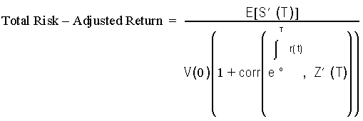
By definition of the total risk-adjusted return for Equation B, we have:
Therefore, by analogy with the previous development,
dS' = (r + m)S' + dM
S(0) = V(0)
This can be decomposed into
dV' = (r + m) V' dt - C' dt + dM'
Equation E
dS' = dV' + dI'
dI' = rI' dt + C' dt
V' (0) - V(0)
The solution of Equation D and Equation F is:
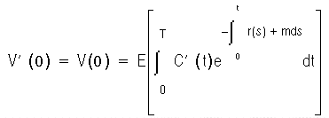
By the law of large numbers, Equation D and Equation F result in:
OAS = m
In other words, the OAS is equal to the risk-adjusted margin.
Related Topics
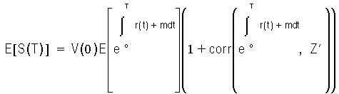
Equivalence of the Static Spread and Margin
Static spread calculations are deterministic. Therefore, they are a special case of the equations in the previous section where all processes generally are equal to their expected value, and the margin p is substituted for the risk-adjusted margin m. The equivalent of Equation C is then:

Here f is the instantaneous forward rate.
The equivalent of Equation D and Equation F is then:
dV' = (r + m)V' dt - C' dt
Equation H
dI' = rI' dt + C' dt
dS' = dV' + dI'
V'(0) = V(0)
The solution of Equation G and Equation I is:
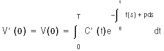
Comparing Equation J and Equation A:
ss = p
In other words, the static spread is equal to the margin.
Related Topics
Option Cost Model Usage Hints
The option cost calculation model is flexible and you can calibrate the calculations to your needs. See:
Related Topics
Overview of Transfer Pricing Option Cost
Nonunicity of the Static Spread
Nonunicity of the static spread means that sometimes more than one value can solve the static-spread equation. However, such cases extremely rare.
Take an instrument with a market value of $0.445495 for example. Suppose the instrument has two cash flows. The following table shows the value of the cash flows and the corresponding discount factors (assuming a static spread of zero).
| Events | Time | Cash Flow Value | Discount Factor (static spread = 0) |
|---|---|---|---|
| First Event | 1 | 1 | 0.9 |
| Second Event | 2 | -0.505025 | 0.8 |
The continuously compounded static spread solves the following equation:
0.9 Exp (-ss) -0.8 * 0.505025 Exp (-2ss) -0.445494 = 0
There are two possible solutions for the static spread:
-
static spread = 0.19%
-
static spread = $1.81
Related Topics
Calibrating the Accuracy of Option Cost Calculations
If you desire a better numerical precision than the default precision, you can take two actions:
-
Decrease the speed factor. See: Calculating Static Spread.
-
Increase the number of Monte Carlo scenarios.
Both actions increase the calculation time.
Related Topics