| Sun Performance Library User's Guide |
| Sun Performance Library User's Guide |
| C H A P T E R 5 |
|
Using Sun Performance Library Signal Processing Routines |
The discrete Fourier transform (DFT) has always been an important analytical tool in many areas in science and engineering. However, it was not until the development of the fast Fourier transform (FFT) that the DFT became widely used. This is because the DFT requires O(N2) computations, while the FFT only requires O(Nlog2N) operations.
Sun Performance Library contains a set of routines that computes the FFT, related FFT operations, such as convolution and correlation, and trigonometric transforms.
This chapter is divided into the following three sections.
Each section includes examples that show how the routines might be used.
For information on the Fortran 95 and C interfaces and types of arguments used in each routine, see the section 3P man pages for the individual routines. For example, to display the man page for the SFFTC routine, type man -s 3P sfftc. Routine names must be lowercase. For an overview of the FFT routines, type man -s 3P fft.
TABLE 5-1 lists the names of the FFT routines and their calling sequence. Double precision routine names are in square brackets. See the individual man pages for detailed information on the data type and size of the arguments.
Sun Performance Library FFT routines use the following arguments.
 for one-dimensional transforms,
 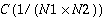 for two-dimensional transforms, and
 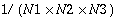 for three-dimensional transforms. In such case, the inverse transform is said to be normalized. If a normalized FFT is followed by its inverse FFT, the result is the original input data. The Sun Performance Library FFT routines are not normalized. However, normalization can be done easily by calling the inverse FFT routine with the appropriate scaling factor stored in SCALE.
Linear FFT routines compute the FFT of real or complex data in one dimension only. The data can be one or more complex or real sequences. For a single sequence, the data is stored in a vector. If more than one sequence is being transformed, the sequences are stored column-wise in a two-dimensional array and a one-dimensional FFT is computed for each sequence along the column direction. The linear forward FFT routines compute
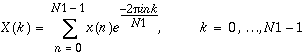
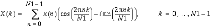
where  , or expressed in polar form,
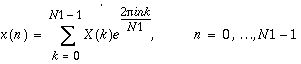
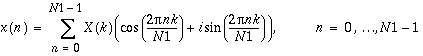
The inverse FFT routines compute
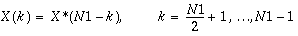
With the forward transform, if the input is one or more complex sequences of size N1, the result will be one or more complex sequences, each consisting of N1 unrelated data points. However, if the input is one or more real sequences, each containing N1 real data points, the result will be one or more complex sequences that are conjugate symmetric. That is,
The imaginary part of X(0) is always zero. If N1 is even, the imaginary part of  is also zero. Both zeros are stored explicitly. Because the second half of each sequence can be derived from the first half, only
  complex data points are computed and stored in the output array. Here and elsewhere in this chapter, integer division is rounded down.
With the inverse transform, if an N1-point complex-to-complex transform is being computed, then N1 unrelated data points are expected in each input sequence and N1 data points will be returned in the output array. However, if an N1-point complex-to-real transform is being computed, only the first  complex data points of each conjugate symmetric input sequence are expected in the input, and the routine will return N1 real data points in each output sequence.
For each value of N1, either the forward or the inverse routine must be called to compute the factors of N1 and the trigonometric weights associated with those factors before computing the actual FFT. The factors and trigonometric weights can be reused in subsequent transforms as long as N1 remains unchanged.
TABLE 5-2 lists the single precision linear FFT routines and their purposes. For routines that have two-dimensional arrays as input and output, TABLE 5-2 also lists the leading dimension requirements. The same information applies to the corresponding double precision routines except that their data types are double precision and double complex. See TABLE 5-2 for the mapping. See the individual man pages for a complete description of the routines and their arguments.
TABLE 5-2 Notes.
CODE EXAMPLE 5-1 shows how to compute the linear real-to-complex and complex-to-real FFT of a set of sequences.
CODE EXAMPLE 5-1 Notes:
The forward FFT of X is actually
Because of symmetry, Z(2) is the complex conjugate of Z(1), and therefore only the first two  complex values are stored. For the in-place forward transform, SFFTCM is called with real array X as the input and output. Because SFFTCM expects the output array to be of type COMPLEX, the leading dimension of X as an output array must be as if X were complex. Since the leading dimension of real array X is LDX = 2 × LDC, the leading dimension of X as a complex output array must be LDC. Similarly, in the in-place inverse transform, CFFTSM is called with complex array Z as the input and output. Because CFFTSM expects the output array to be of type REAL, the leading dimension of Z as an output array must be as if Z were real. Since the leading dimension of complex array Z is LDZ, the leading dimension of Z as a real output array must be LDZ × 2.
CODE EXAMPLE 5-2 shows how to compute the linear complex-to-complex FFT of a set of sequences.
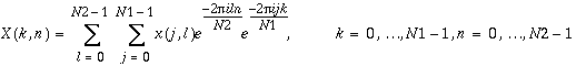
For the linear FFT routines, when the input is a two-dimensional array, the FFT is computed along one dimension only, namely, along the columns of the array. The two-dimensional FFT routines take a two-dimensional array as input and compute the FFT along both the column and row dimensions. Specifically, the forward two-dimensional FFT routines compute
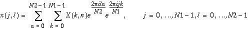
and the inverse two-dimensional FFT routines compute
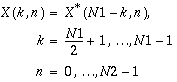
For both the forward and inverse two-dimensional transforms, a complex-to-complex transform where the input problem is N1 × N2 will yield a complex array that is also N1 × N2.
When computing a real-to-complex two-dimensional transform (forward FFT), if the real input array is of dimensions N1 × N2, the result will be a complex array of dimensions  . Conversely, when computing a complex-to-real transform (inverse FFT) of dimensions N1 × N2, an
  complex array is required as input. As with the real-to-complex and complex-to-real linear FFT, because of conjugate symmetry, only the first
  complex data points need to be stored in the input or output array along the first dimension. The complex subarray
 ![X(\frac{N1}{2}+1:N1-1, [:)]](figures/plug_signal_proc-30.gif) can be obtained from
can be obtained from ![X(0:\frac{N1}{2}, [:)]](figures/plug_signal_proc-31.gif) as follows:
as follows:
To compute a two-dimensional transform, an FFT routine must be called twice. One call initializes the routine and the second call actually computes the transform. The initialization includes computing the factors of N1 and N2 and the trigonometric weights associated with those factors. In subsequent forward or inverse transforms, initialization is not necessary as long as N1 and N2 remain unchanged.
IMPORTANT: Upon returning from a two-dimensional FFT routine, Y(0 : N - 1, :) contains the transform results and the original contents of Y(N : LDY-1, :) is overwritten. Here, N = N1 in the complex-to-complex and complex-to-real transforms and N =  in the real-to-complex transform.
TABLE 5-3 lists the single precision two-dimensional FFT routines and their purposes. The same information applies to the corresponding double precision routines except that their data types are double precision and double complex. See TABLE 5-3 for the mapping. Refer to the individual man pages for a complete description of the routines and their arguments.
TABLE 5-3 Notes:
The following example shows how to compute a two-dimensional real-to-complex FFT and complex-to-real FFT of a two-dimensional array.
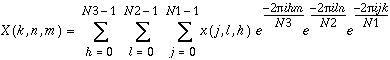
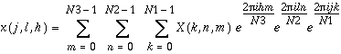
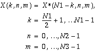
Sun Performance Library includes routines that compute three-dimensional FFT. In this case, the FFT is computed along all three dimensions of a three-dimensional array. The forward FFT computes
In the complex-to-complex transform, if the input problem is N1 × N2 × N3, a three-dimensional transform will yield a complex array that is also N1 × N2 × N3. When computing a real-to-complex three-dimensional transform, if the real input array is of dimensions N1 × N2 × N3, the result will be a complex array of dimensions  . Conversely, when computing a complex-to-real FFT of dimensions N1 × N2 × N3, an
  complex array is required as input. As with the real-to-complex and complex-to-real linear FFT, because of conjugate symmetry, only the first
  complex data points need to be stored along the first dimension. The complex subarray
 ![X(\frac{N1}{2}+1:N1-1,:, [:)]](figures/plug_signal_proc-45.gif) can be obtained from
can be obtained from ![X(0:\frac{N1}{2},:, [:)]](figures/plug_signal_proc-46.gif) as follows:
as follows:
To compute a three-dimensional transform, an FFT routine must be called twice: Once to initialize and once more to actually compute the transform. The initialization includes computing the factors of N1, N2, and N3 and the trigonometric weights associated with those factors. In subsequent forward or inverse transforms, initialization is not necessary as long as N1, N2, and N3 remain unchanged.
IMPORTANT: Upon returning from a three-dimensional FFT routine, Y(0 : N - 1, :, :) contains the transform results and the original contents of Y(N:LDY1-1, :, :) is overwritten. Here, N = N1 in the complex-to-complex and complex-to-real transforms and N =  in the real-to-complex transform.
TABLE 5-4 lists the single precision three-dimensional FFT routines and their purposes. The same information applies to the corresponding double precision routines except that their data types are double precision and double complex. See TABLE 5-4 for the mapping. See the individual man pages for a complete description of the routines and their arguments.
TABLE 5-4 Notes:
CODE EXAMPLE 5-4 shows how to compute the three-dimensional real-to-complex FFT and complex-to-real FFT of a three-dimensional array.
When doing an in-place real-to-complex or complex-to-real transform, care must be taken to ensure the size of the input array is large enough to hold the results. For example, if the input is of type complex stored in a complex array with first leading dimension N, then to use the same array to store the real results, its first leading dimension as a real output array would be 2 × N. Conversely, if the input is of type real stored in a real array with first leading dimension 2 × N, then to use the same array to store the complex results, its first leading dimension as a complex output array would be N. Leading dimension requirements for in-place and out-of-place transforms can be found in TABLE 5-2, TABLE 5-3, and TABLE 5-4.
In the linear and multi-dimensional FFT, the transform between real and complex data through a real-to-complex or complex-to-real transform can be confusing because N1 real data points correspond to  complex data points. N1 real data points do map to N1 complex data points, but because there is conjugate symmetry in the complex data, only
  data points need to be stored as input in the complex-to-real transform and as output in the real-to-complex transform. In the multi-dimensional FFT, symmetry exists along all the dimensions, not just in the first. However, the two-dimensional and three-dimensional FFT routines store the complex data of the second and third dimensions in their entirety.
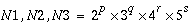
While the FFT routines accept any size of N1, N2 and N3, FFTs can be computed most efficiently when values of N1, N2 and N3 can be decomposed into relatively small primes. A real-to-complex or a complex-to-real transform can be computed most efficiently when
and a complex-to-complex transform can be computed most efficiently when
where p, q, r, s, t, u, and v are integers and p, q, r, s, t, u, v  0.
0.
The function xFFTOPT can be used to determine the optimal sequence length, as shown in CODE EXAMPLE 5-5.
Input to the DFT that possess special symmetries occur in various applications. A transform that exploits symmetry usually saves in storage and computational count, such as with the real-to-complex and complex-to-real FFT transforms. The Sun Performance Library cosine and sine transforms are special cases of FFT routines that take advantage of the symmetry properties found in even and odd functions.
|
Note - Sun Performance Library sine and cosine transform routines are based on the routines contained in FFTPACK (http://www.netlib.org/fftpack/). Routines with a V prefix are vectorized routines that are based on the routines contained in VFFTPACK (http://www.netlib.org/vfftpack/). |
TABLE 5-5 lists the Sun Performance Library fast cosine and sine transforms. Names of double precision routines are in square brackets. Routines whose name begins with 'V' can compute the transform of one or more sequences simultaneously. Those whose name ends with 'I' are initialization routines.
TABLE 5-5 Notes:
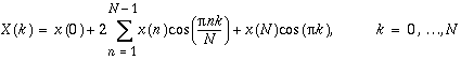
A special form of the FFT that operates on real even sequences is the fast cosine transform (FCT). A real sequence x is said to have even symmetry if x(n) = x(-n) where n = -N + 1, ..., 0, ..., N. An FCT of a sequence of length 2N requires N + 1 input data points and produces a sequence of size N + 1. Routine COST computes the FCT of a single real even sequence while VCOST computes the FCT of one or more sequences. Before calling [V]COST, [V]COSTI must be called to compute trigonometric constants and factors associated with input length N + 1. The FCT is its own inverse transform. Calling VCOST twice will result in the original N +1 data points. Calling COST twice will result in the original N +1 data points multiplied by 2N.
An even sequence x with symmetry such that x(n) = x(-n - 1) where n = -N + 1, ... , 0, ..., N is said to have quarter-wave even symmetry. COSQF and COSQB compute the FCT and its inverse, respectively, of a single real quarter-wave even sequence. VCOSQF and VCOSQB operate on one or more sequences. The results of [V]COSQB are unormalized, and if scaled by  , the original sequences are obtained. An FCT of a real sequence of length 2N that has quarter-wave even symmetry requires N input data points and produces an N-point resulting sequence. Initialization is required before calling the transform routines by calling [V]COSQI.
Another type of symmetry that is commonly encountered is the odd symmetry where x(n) = -x(-n) for n = -N+1, ..., 0, ..., N. As in the case of the fast cosine transform, the fast sine transform (FST) takes advantage of the odd symmetry to save memory and computation. For a real odd sequence x, symmetry implies that x(0) = -x(0) = 0. Therefore, if x is of length 2N then only N = 1 values of x are required to compute the FST. Routine SINT computes the FST of a single real odd sequence while VSINT computes the FST of one or more sequences. Before calling [V]SINT, [V]SINTI must be called to compute trigonometric constants and factors associated with input length N - 1. The FST is its own inverse transform. Calling VSINT twice will result in the original N -1 data points. Calling SINT twice will result in the original N -1 data points multiplied by 2N.
An odd sequence with symmetry such that x(n) = -x(-n - 1), where
n = -N + 1, ..., 0, ..., N is said to have quarter-wave odd symmetry. SINQF and SINQB compute the FST and its inverse, respectively, of a single real quarter-wave odd sequence while VSINQF and VSINQB operate on one or more sequences. SINQB is unnormalized, so using the results of SINQF as input in SINQB produces the original sequence scaled by a factor of 4N. However, VSINQB is normalized, so a call to VSINQF followed by a call to VSINQB will produce the original sequence. An FST of a real sequence of length 2N that has quarter-wave odd symmetry requires N input data points and produces an N-point resulting sequence. Initialization is required before calling the transform routines by calling [V]SINQI.
Sun Performance Library routines use the equations in the following sections to compute the fast cosine and sine transforms and inverse transforms.
The forward and inverse FCT of a sequence is computed as
 .
.
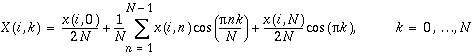
The forward and inverse FCTs of multiple sequences are computed as
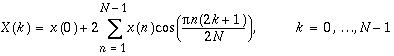
The forward FCT of a quarter-wave even sequence is computed as
N values are needed to compute the forward FCT of an N-point quarter-wave even sequence.
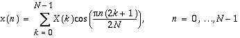
The inverse FCT of a quarter-wave even sequence is computed as
Calling the forward and inverse routines will result in the original input scaled by  .
.
The forward FCT of one or more quarter-wave even sequences is computed as
The inverse FCT of one or more quarter-wave even sequences is computed as
The forward and inverse FST of a sequence is computed as
 .
.
The forward and inverse fast sine transforms of multiple sequences are computed as
The forward FST of a quarter-wave odd sequence is computed as
N values are needed to compute the forward FST of an N-point quarter-wave odd sequence.
The inverse FST of a quarter-wave odd sequence is computed as
Calling the forward and inverse routines will result in the original input scaled by  .
.
The forward FST of one or more quarter-wave odd sequences is computed as
The inverse FST of one or more quarter-wave odd sequences is computed as
CODE EXAMPLE 5-6 calls COST to compute the FCT and the inverse transform of a real even sequence. If the real sequence is of length 2N, only N + 1 input data points need to be stored and the number of resulting data points is also N + 1. The results are stored in the input array.
CODE EXAMPLE 5-7 calls VCOSQF and VCOSQB to compute the FCT and the inverse FCT, respectively, of two real quarter-wave even sequences. If the real sequences are of length 2N, only N input data points need to be stored, and the number of resulting data points is also N. The results are stored in the input array.
In CODE EXAMPLE 5-8, SINT is called to compute the FST and the inverse transform of a real odd sequence. If the real sequence is of length 2N, only N - 1 input data points need to be stored and the number of resulting data points is also N - 1. The results are stored in the input array.
In CODE EXAMPLE 5-9 VSINQF and VSINQB are called to compute the FST and inverse FST, respectively, of two real quarter-wave odd sequences. If the real sequence is of length 2N, only N input data points need to be stored and the number of resulting data points is also N. The results are stored in the input array.
Two applications of the FFT that are frequently encountered especially in the signal processing area are the discrete convolution and discrete correlation operations.
Given two functions x(t) and y(t), the Fourier transform of the convolution of x(t) and y(t), denoted as x  y, is the product of their individual Fourier transforms: DFT(x
  y)=X
y)=X Y where
  denotes the convolution operation and
  denotes pointwise multiplication.
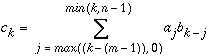
Typically, x(t) is a continuous and periodic signal that is represented discretely by a set of N data points xj, j = 0, ..., N -1, sampled over a finite duration, usually for one period of x(t) at equal intervals. y(t) is usually a response that starts out as zero, peaks to a maximum value, and then returns to zero. Discretizing y(t) at equal intervals produces a set of N data points, yk, k = 0, ..., N -1. If the actual number of samplings in yk is less than N, the data can be padded with zeros. The discrete convolution can then be defined as
The values of  , are the same as those of
  but in the wrap-around order.
The Sun Performance Library routines allow the user to compute the convolution by using the definition above with k = 0, ..., N -1, or by using the FFT. If the FFT is used to compute the convolution of two sequences, the following steps are performed:
One interesting characteristic of convolution is that the product of two polynomials is actually a convolution. A product of an m-term polynomial
has m + n - 1 coefficients that can be obtained by
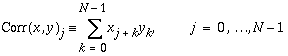
Closely related to convolution is the correlation operation. It computes the correlation of two sequences directly superposed or when one is shifted relative to the other. As with convolution, we can compute the correlation of two sequences efficiently as follows using the FFT:
The routines in the Performance Library also allow correlation to be computed by the following definition:
There are various ways to interpret the sampled input data of the convolution and correlation operations. The argument list of the convolution and correlation routines contain parameters to handle cases in which
Sun Performance Library contains the convolution routines shown in TABLE 5-6.
The [S,D,C,Z]CNVCOR routines are used to compute the convolution or correlation of a filter with one or more input vectors. The [S,D,C,Z]CNVCOR2 routines are used to compute the two-dimensional convolution or correlation of two matrices.
The one-dimensional convolution and correlation routines use the arguments shown in TABLE 5-7.
|
`V' or `v' specifies that convolution is computed.
|
|
|
`T' or `t' specifies that the Fourier transform method is used.
|
|
|
Number of implicit zeros prefixed to the Y vectors, where NPRE |
|
|
Stride between elements of the input vectors in Y, where INC1Y > 0. |
|
|
Number of Z vectors, where K |
|
|
Stride between elements of the output vectors in Z, where INCYZ > 0. |
|
The two-dimensional convolution and correlation routines use the arguments shown in TABLE 5-8.
|
`V' or `v' specifies that convolution is computed.
|
|
|
`T' or `t' specifies that the Fourier transform method is used.
|
|
|
`N' or `n' specifies that X is the filter matrix
|
|
|
`N' or `n' specifies that X must be preserved
|
|
|
`N' or `n' specifies that Y is the input matrix
|
|
|
`N' or `n' specifies that Y must be preserved
|
|
|
Filter matrix. X is unchanged on exit when SCRATCHX is `N' or `n' and undefined on exit when SCRATCHX is `S' or `s'. |
|
|
Number of implicit zeros prefixed to each row of the input matrix Y vectors, where MPRE |
|
|
Number of implicit zeros prefixed to each column of the input matrix Y, where NPRE |
|
|
Input matrix. Y is unchanged on exit when SCRATCHY is `N' or `n' and undefined on exit when SCRATCHY is `S' or `s'. |
|
|
Leading dimension of the array containing the result matrix Z, where LDZ |
|
The minimum dimensions for the WORK work arrays used with the one-dimensional and two-dimensional convolution and correlation routines are shown in TABLE 5-11. The minimum dimensions for one-dimensional convolution and correlation routines depend upon the values of the arguments NPRE, NX, NY, and NZ.
The minimum dimensions for two-dimensional convolution and correlation routines depend upon the values of the arguments shown TABLE 5-9.
|
Number of implicit zeros prefixed to each row of the input matrix |
|
|
Number of implicit zeros prefixed to each column of the input matrix |
|
|
MPRE + MPOST + MYC_INIT, where MYC_INIT depends upon filter and input matrices, as shown in TABLE 5-10 |
|
|
NPRE + NPOST + NYC_INIT, where NYC_INIT depends upon filter and input matrices, as shown in TABLE 5-10 |
MYC_INIT and NYC_INIT depend upon the following, where X is the filter matrix and Y is the input matrix.
The values assigned to the minimum work array size is shown in TABLE 5-11.
|
SCNVCOR2[3], DCNVCOR21 |
||
CODE EXAMPLE 5-10 uses CCNVCOR to perform FFT convolution of two complex vectors.
If any vector overlaps a writable vector, either because of argument aliasing or ill-chosen values of the various INC arguments, the results are undefined and can vary from one run to the next.
The most common form of the computation, and the case that executes fastest, is applying a filter vector X to a series of vectors stored in the columns of Y with the result placed into the columns of Z. In that case, INCX = 1, INC1Y = 1, INC2Y NY, INC1Z = 1, INC2Z NZ. Another common form is applying a filter vector X to a series of vectors stored in the rows of Y and store the result in the row of Z, in which case INCX = 1, INC1Y NY, INC2Y = 1, INC1Z NZ, and INC2Z = 1.
Convolution can be used to compute the products of polynomials. CODE EXAMPLE 5-11 uses SCNVCOR to compute the product of 1 + 2x + 3x2 and 4 + 5x + 6x2.
Making the output vector longer than the input vectors, as in the example above, implicitly adds zeros to the end of the input. No zeros are actually required in any of the vectors, and none are used in the example, but the padding provided by the implied zeros has the effect of an end-off shift rather than an end-around shift of the input vectors.
CODE EXAMPLE 5-12 will compute the product between the vector [ 1, 2, 3 ] and the circulant matrix defined by the initial column vector [ 4, 5, 6 ].
The difference between this example and the previous example is that the length of the output vector is the same as the length of the input vectors, so there are no implied zeros on the end of the input vectors. With no implied zeros to shift into, the effect of an end-off shift from the previous example does not occur and the end-around shift results in a circulant matrix product.
For additional information on the DFT or FFT, see the following sources.
Briggs, William L., and Henson, Van Emden. The DFT: An Owner's Manual for the Discrete Fourier Transform. Philadelphia, PA: SIAM, 1995.
Brigham, E. Oran. The Fast Fourier Transform and Its Applications. Upper Saddle River, NJ: Prentice Hall, 1988.
Chu, Eleanor, and George, Alan. Inside the FFT Black Box: Serial and Parallel Fast Fourier Transform Algorithms. Boca Raton, FL: CRC Press, 2000.
Press, William H., Teukolsky, Saul A., Vetterling, William T., and Flannery, Brian P. Numerical Recipes in C: The Art of Scientific Computing. 2 ed. Cambridge, United Kingdom: Cambridge University Press, 1992.
Press, William H., Teukolsky, Saul A., Vetterling, William T., and Flannery, Brian P. Numerical Recipes in Fortran: The Art of Scientific Computing. 2 ed. Cambridge, United Kingdom: Cambridge University Press, 1992.
Ramirez, Robert W. The FFT: Fundamentals and Concepts. Englewood Cliffs, NJ: Prentice-Hall, Inc., 1985.
Swartzrauber, Paul N. Vectorizing the FFTs. In Rodrigue, Garry ed. Parallel Computations. New York: Academic Press, Inc., 1982.
Strang, Gilbert. Linear Algebra and Its Applications. 3 ed. Orlando, FL: Harcourt Brace & Company, 1988.
Van Loan, Charles. Computational Frameworks for the Fast Fourier Transform. Philadelphia, PA: SIAM, 1992.
Walker, James S. Fast Fourier Transforms. Boca Raton, FL: CRC Press, 1991.
| Sun Performance Library User's Guide | 816-2463-10 |
Copyright © 2002, Sun Microsystems, Inc. All rights reserved.

 ,
, .
. ,
, .
. .
. ,
,
 ,
,
 ,
,
 ,
,


 ,
, .
.
 ,
,


 ,
,


 ,
, ,
,
 ,
,


 ,
,


 ,
, ,
, .
. .
. .
. .
.![X(i,k)=\frac{1}{N}\left[ x(i,0)+2\sum _{n=1}^{N-1}x(i,n)\cos (\frac{\pi n(2k+1)}{2N})\right] , k=0,\ldots N-1](figures/plug_signal_proc-67.gif) .
. .
. .
. .
. .
. .
.![X(i,k)=\frac{1}{\sqrt{4N}}\left[ 2\sum _{n=0}^{N-2}x(n,i)\sin (\frac{\pi (n+1)(2k+1)}{2N})+x(N-1,i)\cos (\pi k)\right] , k=0,\ldots N-1](figures/plug_signal_proc-75.gif) .
.
 .
. y)j
y)j .
.
 DFT(x
DFT(x  y)
y)
 y)
y)
 ,
, .
.