Release 2 (8.1.6)
A76989-01
Library |
Product |
Contents |
Index |
| Oracle8i SQL Reference Release 2 (8.1.6) A76989-01 |
|
![]()
![]()
![]()
Functions, 75 of 121
The linear regression functions are:
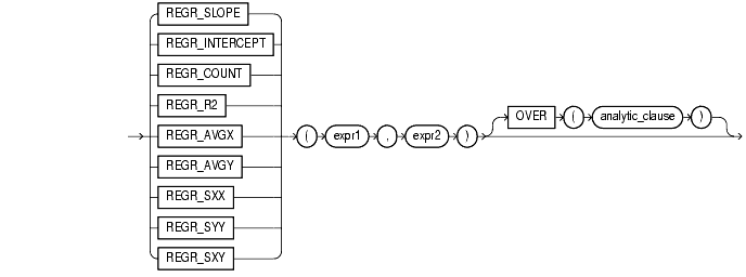
For information on syntax and semantics, see "Analytic Functions".
The linear regression functions fit an ordinary-least-squares regression line to a set of number pairs. You can use them as both aggregate and analytic functions.
Oracle applies the function to the set of (expr1, expr2) pairs after eliminating all pairs for which either expr1 or expr2 is null. Oracle computes all the regression functions simultaneously during a single pass through the data.
expr1 is interpreted as a value of the dependent variable (a "y value"), and expr2 is interpreted as a value of the independent variable (an "x value"). Both expressions must be numbers.
REGR_SLOPE returns the slope of the line. The return value is a number and can be null. After the elimination of null (expr1, expr2) pairs, it makes the following computation:
COVAR_POP(expr1, expr2) / VAR_POP(expr2)
REGR_INTERCEPT returns the y-intercept of the regression line. The return value is a number and can be null. After the elimination of null (expr1, expr2) pairs, it makes the following computation:
AVG(expr1) - REGR_SLOPE(expr1, expr2) * AVG(expr2)
REGR_COUNT returns an integer that is the number of non-null number pairs used to fit the regression line.
REGR_R2 returns the coefficient of determination (also called "R-squared" or "goodness of fit") for the regression. The return value is a number and can be null. VAR_POP(expr1) and VAR_POP(expr2) are evaluated after the elimination of null pairs. The return values are:
                     NULL if VAR_POP(expr2)  = 0

                        1 if VAR_POP(expr1)  = 0 and
                             VAR_POP(expr2) != 0

POWER(CORR(expr1,expr),2) if VAR_POP(expr1)  > 0 and
                             VAR_POP(expr2  != 0
All of the remaining regression functions return a number and can be null:
REGR_AVGX evaluates the average of the independent variable (expr2) of the regression line. It makes the following computation after the elimination of null (expr1, expr2) pairs:
AVG(expr2)
REGR_AVGY evaluates the average of the dependent variable (expr1) of the regression line. It makes the following computation after the elimination of null (expr1, expr2) pairs:
AVG(expr1)
REGR_SXY, REGR_SXX, REGR_SYY are auxiliary functions that are used to compute various diagnostic statistics.
REGR_SXX makes the following computation after the elimination of null (expr1, expr2) pairs:
REGR_COUNT(expr1, expr2) * VAR_POP(expr2)
REGR_SYY makes the following computation after the elimination of null (expr1, expr2) pairs:
REGR_COUNT(expr1, expr2) * VAR_POP(expr1)
REGR_SXY makes the following computation after the elimination of null (expr1, expr2) pairs:
REGR_COUNT(expr1, expr2) * COVAR_POP(expr1, expr2)
The following examples are based on the SALES table, described in "COVAR_POP".
The following example determines the slope and intercept of the regression line for the amount of sales and sale profits for each year.
SELECT s_year,
   REGR_SLOPE(s_amount, s_profit),
   REGR_INTERCEPT(s_amount, s_profit)
FROM sales GROUP BY s_year;

 S_YEAR     REGR_SLOPE REGR_INTER
---------- ---------- ----------
      1998 128.401558 -2277.5684
      1999  55.618655 226.855296
The following example determines the cumulative slope and cumulative intercept of the regression line for the amount of sales and sale profits for each day in 1998:
SELECT s_year, s_month, s_day,
   REGR_SLOPE(s_amount, s_profit)
      OVER (ORDER BY s_month, s_day) AS CUM_SLOPE,
   REGR_INTERCEPT(s_amount, s_profit)
      OVER (ORDER BY s_month, s_day) AS CUM_ICPT
   FROM sales
   WHERE s_year=1998
   ORDER BY s_month, s_day;

S_YEAR     S_MONTH    S_DAY      CUM_SLOPE  CUM_ICPT
---------- ---------- ---------- ---------- ----------
      1998          6          5
      1998          6          9 132.093066 401.884833
      1998          6          9 132.093066 401.884833
      1998          6         10 131.829612  450.65349
      1998          8         21 132.963737  -153.5413
      1998          8         25 130.681718 -451.47349
      1998          8         25 130.681718 -451.47349
      1998          8         26  128.76502 -236.50096
      1998         11          9 131.499934 -1806.7535
      1998         11          9 131.499934 -1806.7535
      1998         11         10 130.190972 -2323.3056
      1998         11         10 130.190972 -2323.3056
      1998         11         11 128.401558 -2277.5684
The following example returns the number of sales transactions in the SALES table that resulted in a profit. (None of the rows for containing a sales amount have a null in the S_PROFIT column, so the function returns the total number of rows in the SALES table.)
SELECT REGR_COUNT(s_amount, s_profit) FROM sales;

REGR_COUNT
----------
        23
The following example computes, for each day, the cumulative number of transactions within each month for the year 1998:
SELECT s_month, s_day,
   REGR_COUNT(s_amount,s_profit)
      OVER (PARTITION BY s_month ORDER BY s_day)
FROM SALES
WHERE S_YEAR=1998
ORDER BY S_MONTH;

S_MONTH    S_DAY      REGR_COUNT
---------- ---------- ----------
         6          5          1
         6          9          3
         6          9          3
         6         10          4
         8         21          1
         8         25          3
         8         25          3
         8         26          4
        11          9          2
        11          9          2
        11         10          4
        11         10          4
        11         11          5
The following example computes the coefficient of determination of the regression line for amount of sales and sale profits:
SELECT REGR_R2(s_amount, s_profit) FROM sales;

REGR_R2(S_
----------
.942435028
The following example computes the cumulative coefficient of determination of the regression line for monthly sales and monthly profits for each month in 1998:
SELECT s_month,
       REGR_R2(SUM(s_amount), SUM(s_profit))
              OVER (ORDER BY s_month)
FROM SALES
WHERE s_year=1998
GROUP BY s_month
ORDER BY s_month;

S_MONTH    REGR_R2(SU
---------- ----------
         6
         8          1
        11 .740553632
The following example calculates the regression average for the amount of sales and sale profits for each year:
SELECT s_year,
   REGR_AVGY(s_amount, s_profit),
   REGR_AVGX(s_amount, s_profit)
FROM sales GROUP BY s_year;

 S_YEAR     REGR_AVGY( REGR_AVGX(
---------- ---------- ----------
      1998 41227.5462 338.820769
      1999   7330.748    127.725
The following example calculates the cumulative averages for the amount of sales and sale profits in 1998:
SELECT s_year, s_month, s_day,
   REGR_AVGY(s_amount, s_profit)
      OVER (ORDER BY s_month, s_day) AS CUM_AMOUNT,
   REGR_AVGX(s_amount, s_profit)
      OVER (ORDER BY s_month, s_day) AS CUM_PROFIT
   FROM sales
   WHERE s_year=1998
   ORDER BY s_month, s_day;

S_YEAR     S_MONTH    S_DAY      CUM_AMOUNT CUM_PROFIT
---------- ---------- ---------- ---------- ----------
      1998          6          5      16068      118.2
      1998          6          9 44375.6667      332.9
      1998          6          9 44375.6667      332.9
      1998          6         10   52678.25    396.175
      1998          8         21   44721.72      337.5
      1998          8         25    45333.8 350.357143
      1998          8         25    45333.8 350.357143
      1998          8         26    47430.7   370.1875
      1998         11          9   41892.91    332.317
      1998         11          9   41892.91    332.317
      1998         11         10  40777.175 331.055833
      1998         11         10  40777.175 331.055833
      1998         11         11 41227.5462 338.820769
The following example computes the REGR_SXY, REGR_SXX, and REGR_SYY values for the regression analysis of amount of sales and sale profits for each year:
SELECT s_year,
   REGR_SXY(s_amount, s_profit),
       REGR_SYY(s_amount, s_profit),
       REGR_SXX(s_amount, s_profit)
FROM sales GROUP BY s_year;

S_YEAR     REGR_SXY(S REGR_SYY(S REGR_SXX(S
---------- ---------- ---------- ----------
      1998 48723551.8 6423698688 379462.311
      1999 3605361.62  200525751 64822.8841
The following example computes the cumulative REGR_SXY, REGR_SXX, and REGR_SYY statistics for amount of sales and sale profits for each month-day value in 1998:
SELECT s_year, s_month, s_day,
       REGR_SXY(s_amount, s_profit)
              OVER (ORDER BY s_month, s_day) AS CUM_SXY,
       REGR_SYY(s_amount, s_profit)
              OVER (ORDER BY s_month, s_day) AS CUM_SXY,
       REGR_SXX(s_amount, s_profit)
              OVER (ORDER BY s_month, s_day) AS CUM_SXX
   FROM sales
   WHERE s_year=1998
   ORDER BY s_month, s_day;

S_YEAR     S_MONTH    S_DAY      CUM_SXY    CUM_SXY    CUM_SXX
---------- ---------- ---------- ---------- ---------- ----------
      1998          6          5          0          0          0
      1998          6          9 14822857.8 1958007601  112215.26
      1998          6          9 14822857.8 1958007601  112215.26
      1998          6         10 21127009.3 2785202281 160259.968
      1998          8         21 30463997.3 4051329674  229115.08
      1998          8         25 34567985.3 4541739739 264520.437
      1998          8         25 34567985.3 4541739739 264520.437
      1998          8         26 36896592.7 4787971157 286542.049
      1998         11          9 45567995.3 6045196901 346524.854
      1998         11          9 45567995.3 6045196901 346524.854
      1998         11         10 48178003.8 6392056557 370056.411
      1998         11         10 48178003.8 6392056557 370056.411
      1998         11         11 48723551.8 6423698688 379462.311
|
|
 Copyright © 1999 Oracle Corporation. All Rights Reserved. |
|