Release 2 (9.2)
Part Number A96533-01
 Home |
 Book List |
 Contents |
 Index |
 Master Index |
 Feedback |
| Oracle9i Database Performance Tuning Guide and Reference Release 2 (9.2) Part Number A96533-01 |
|
This chapter discusses SQL processing, optimization methods, and how the optimizer chooses to execute SQL statements.
The chapter contains the following sections:
The SQL processing architecture contains the following main components:
Figure 1-1 illustrates the SQL processing architecture:
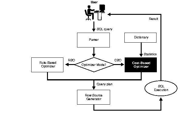
The parser, the optimizer, and the row source generator form the SQL Compiler. The SQL Compiler compiles the SQL statements into a shared cursor, which is associated with the execution plan.
The parser performs two functions:
The optimizer uses internal rules or costing methods to determine the most efficient way of producing the result of the query. The output from the optimizer is a plan that describes an optimum method of execution. The Oracle server provides two methods of optimization: cost-based optimizer (CBO) and rule-based optimizer (RBO).
|
Note: Oracle Corporation strongly advises the use of cost-based optimization. Rule-based optimization will be deprecated in a future release. |
The row source generator receives the optimal plan from the optimizer. It outputs the execution plan for the SQL statement. The execution plan is a collection of row sources structured in the form of a tree. Each row source returns a set of rows for that step.
The SQL execution engine is the component that operates on the execution plan associated with a SQL statement. It then produces the results of the query. Each row source produced by the row source generator is executed by the SQL execution engine.
The optimizer determines the most efficient way to execute a SQL statement. This determination is an important step in the processing of any SQL statement. Often, a SQL statement can be executed in many different ways; for example, tables or indexes can be accessed in a different order. The way Oracle executes a statement can greatly affect execution time.
The optimizer considers many factors related to the objects referenced and the conditions specified in the query. It can use either a cost-based or a rule-based approach.
You can influence the optimizer's choices by setting the optimizer approach and goal, and by gathering representative statistics for the CBO. Sometimes, the application designer, who has more information about a particular application's data than is available to the optimizer, can choose a more effective way to execute a SQL statement. The application designer can use hints in SQL statements to specify how the statement should be executed.
See Also:
|
For any SQL statement processed by Oracle, the optimizer performs the following operations:
| Operation | Description |
|---|---|
|
The optimizer first evaluates expressions and conditions containing constants as fully as possible. (See "How the Optimizer Performs Operations".) |
|
|
For complex statements involving, for example, correlated subqueries or views, the optimizer might transform the original statement into an equivalent join statement. (See "How the Optimizer Transforms SQL Statements".) |
|
|
The optimizer chooses either a cost-based or rule-based approach and determines the goal of optimization. (See "Choosing an Optimizer Approach and Goal".) |
|
|
For each table accessed by the statement, the optimizer chooses one or more of the available access paths to obtain table data. (See "Understanding Access Paths for the CBO".) |
|
|
For a join statement that joins more than two tables, the optimizer chooses which pair of tables is joined first, and then which table is joined to the result, and so on. |
|
|
For any join statement, the optimizer chooses an operation to use to perform the join. See "How the CBO Chooses the Join Method".) |
To execute a DML statement, Oracle might need to perform many steps. Each of these steps either retrieves rows of data physically from the database or prepares them in some way for the user issuing the statement. The combination of the steps Oracle uses to execute a statement is called an execution plan. An execution plan includes an access path for each table that the statement accesses and an ordering of the tables (the join order) with the appropriate join method.
You can examine the execution plan chosen by the optimizer for a SQL statement by using the EXPLAIN PLAN statement. When the statement is issued, the optimizer chooses an execution plan and then inserts data describing the plan into a database table. Simply issue the EXPLAIN PLAN statement and then query the output table.
Example 1-1 uses EXPLAIN PLAN to examine a SQL statement that selects the name, job, salary, and department name for all employees whose salaries do not fall into a recommended salary range.
EXPLAIN PLAN FOR
SELECT employee_id, job_id, salary, department_name
FROM employees, departments
WHERE employees.department_id = departments.department_id
AND NOT EXISTS


(SELECT *
FROM jobs
WHERE employees.salary BETWEEN min_salary AND max_salary);
The resulting output table shows the execution plan chosen by the optimizer to execute the SQL statement in the example:
ID    OPERATION           OPTIONS        OBJECT_NAME
------------------------------------------------------------
0     SELECT STATEMENT
1       FILTER
2         NESTED LOOPS
3           TABLE ACCESS  FULL           EMPLOYEES
4           TABLE ACCESS  BY ROWID       DEPARTMENTS
5             INDEX       UNIQUE SCAN    PK_DEPARTMENT_ID
6         TABLE ACCESS    FULL           JOBS
Figure 1-2 shows a graphical representation of the execution plan for this SQL statement.
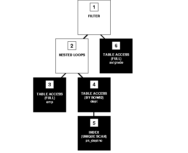
Each box in Figure 1-2 and each row in the output table corresponds to a single step in the execution plan. For each row in the listing, the value in the ID column is the value shown in the corresponding box in Figure 1-2.
Each step of the execution plan returns a set of rows that either is used by the next step or, in the last step, is returned to the user or application issuing the SQL statement. A set of rows returned by a step is called a row set.
Figure 1-2 is a hierarchical diagram showing the flow of row sources from one step to another. The numbering of the steps reflects the order in which they are displayed in response to the EXPLAIN PLAN statement. Generally, the display order is not the same as the order in which the steps are executed.
Each step of the execution plan either retrieves rows from the database or accepts rows from one or more row sources as input:
employees and jobs tables, respectively.department_id value in the pk_department_id index returned by Step 3. It finds the rowids of the associated rows in the departments table.departments table.See Also:
|
The steps of the execution plan are not performed in the order in which they are numbered. Rather, Oracle first performs the steps that appear as leaf nodes in the tree-structured graphical representation of the execution plan (Steps 3, 5, and 6 in Figure 1-2). The rows returned by each step become the row sources of its parent step. Then, Oracle performs the parent steps.
For example, Oracle performs the following steps to execute the statement in Figure 1-2:
Oracle performs Steps 5, 4, 2, 6, and 1 once for each row returned by Step 3. If a parent step requires only a single row from its child step before it can be executed, then Oracle performs the parent step as soon as a single row has been returned from the child step. If the parent of that parent step also can be activated by the return of a single row, then it is executed as well.
Thus, statement execution can cascade up the tree, possibly to encompass the rest of the execution plan. Oracle performs the parent step and all cascaded steps once for each row retrieved by the child step. The parent steps that are triggered for each row returned by a child step include table accesses, index accesses, nested loop joins, and filters.
If a parent step requires all rows from its child step before it can be executed, then Oracle cannot perform the parent step until all rows have been returned from the child step. Such parent steps include sorts, sort merge joins, and aggregate functions.
By default, the goal of the CBO is the best throughput. This means that it chooses the least amount of resources necessary to process all rows accessed by the statement.
Oracle can also optimize a statement with the goal of best response time. This means that it uses the least amount of resources necessary to process the first row accessed by a SQL statement.
The execution plan produced by the optimizer can vary depending on the optimizer's goal. Optimizing for best throughput is more likely to result in a full table scan rather than an index scan, or a sort merge join rather than a nested loop join. Optimizing for best response time, however, more likely results in an index scan or a nested loop join.
For example, suppose you have a join statement that can be executed with either a nested loops operation or a sort-merge operation. The sort-merge operation might return the entire query result faster, while the nested loops operation might return the first row faster. If your goal is to improve throughput, then the optimizer is more likely to choose a sort merge join. If your goal is to improve response time, then the optimizer is more likely to choose a nested loop join.
Choose a goal for the optimizer based on the needs of your application:
The optimizer's behavior when choosing an optimization approach and goal for a SQL statement is affected by the following factors:
The OPTIMIZER_MODE initialization parameter establishes the default behavior for choosing an optimization approach for the instance. It can have the following values:
For example: The following statement changes the goal of the CBO for the session to best response time:
ALTER SESSION SET OPTIMIZER_MODE = FIRST_ROWS_10;
If the optimizer uses the cost-based approach for a SQL statement, and if some tables accessed by the statement have no statistics, then the optimizer uses internal information (such as the number of data blocks allocated to these tables) to estimate other statistics for these tables.
The OPTIMIZER_GOAL parameter of the ALTER SESSION statement can override the optimizer approach and goal established by the OPTIMIZER_MODE initialization parameter for an individual session.
The value of this parameter affects the optimization of SQL statements issued by the user, including those issued by stored procedures and functions called during the session. It does not affect the optimization of internal recursive SQL statements that Oracle issues during the session for operations such as space management and data dictionary operations.
The OPTIMIZER_GOAL parameter can have the same values as the OPTIMIZER_MODE initialization parameter
Any of the following hints in an individual SQL statement can override the OPTIMIZER_MODE initialization parameter and the OPTIMIZER_GOAL parameter of the ALTER SESSION statement:
By default, the cost-based approach optimizes for best throughput. You can change the goal of the CBO in the following ways:
ALTER SESSION SET OPTIMIZER_MODE statement with the ALL_ROWS, FIRST_ROWS, or FIRST_ROWS_n (where n = 1, 10, 100, or 1000) clause.ALL_ROWS, FIRST_ROWS(n ) (where n = any positive integer), or FIRST_ROWS hint.
| See Also:
Chapter 5, "Optimizer Hints" for information on how to use hints |
The statistics used by the CBO are stored in the data dictionary. You can collect exact or estimated statistics about physical storage characteristics and data distribution in these schema objects by using the DBMS_STATS package or the ANALYZE statement.
To maintain the effectiveness of the CBO, you must have statistics that are representative of the data. You can gather statistics on objects in either of the following ways:
DBMS_STATS package.ANALYZE statement.For table columns that contain skewed data (in other words, values with large variations in number of duplicates), you should collect histograms.
The resulting statistics provide the CBO with information about data uniqueness and distribution. Using this information, the CBO is able to compute plan costs with a high degree of accuracy. This enables the CBO to choose the best execution plan based on the least cost.
|
Note: Oracle Corporation strongly recommends that you use the However, you must use the |
The CBO can optimize a SQL statement either for throughput or for fast response. Fast-response optimization is used when the parameter OPTIMIZER_MODE is set to FIRST_ROWS_n (where n is 1, 10, 100, or 1000) or FIRST_ROWS. A hint FIRST_ROWS(n ) (where n is any positive integer) or FIRST_ROWS can be used to optimize an individual SQL statement for fast response. Fast-response optimization is suitable for online users, such as those using Oracle Forms or Web access. Typically, online users are interested in seeing the first few rows; they seldom look at the entire query result, especially when the result size is large. For such users, it makes sense to optimize the query to produce the first few rows as quickly as possible, even if the time to produce the entire query result is not minimized.
With fast-response optimization, the CBO generates a plan with the lowest cost to produce the first row or the first few rows. The CBO employs two different fast-response optimizations, referred to here as the old and new methods. The old method is used with the FIRST_ROWS hint or parameter value. With the old method, the CBO uses a mixture of costs and rules to produce a plan. It is retained for backward compatibility reasons.
The new fast-response optimization method is used with either the FIRST_ROWS_n parameter value (where n can be 1, 10, 100, or 1000) or with the FIRST_ROWS(n) hint (where n can be any positive integer). The new method is totally based on costs, and it is sensitive to the value of n. With small values of n, the CBO tends to generate plans that consist of nested loop joins with index lookups. With large values of n, the CBO tends to generate plans that consist of hash joins and full table scans.
The value of n should be chosen based on the online user requirement and depends specifically on how the result is displayed to the user. Generally, Oracle Forms users see the result one row at a time and they are typically interested in seeing the first few screens. Other online users see the result one group of rows at a time.
With the fast-response method, the CBO explores different plans and computes the cost to produce the first n rows for each. It picks the plan that produces the first n rows at lowest cost. Remember that with fast-response optimization, a plan that produces the first n rows at lowest cost might not be the optimal plan to produce the entire result. If the requirement is to obtain the entire result of a query, then fast-response optimization should not be used. Instead use the ALL_ROWS parameter value or hint.
The following features require use of the CBO:
SAMPLE clauses in a SELECT statementIn general, use the cost-based approach. Oracle Corporation is continually improving the CBO, and new features require it. The rule-based approach is available for backward compatibility with legacy applications.
The CBO determines which execution plan is most efficient by considering available access paths and by factoring in information based on statistics for the schema objects (tables or indexes) accessed by the SQL statement. The CBO also considers hints, which are optimization suggestions placed in a comment in the statement.
| See Also:
Chapter 5, "Optimizer Hints" for detailed information on hints |
The CBO performs the following steps:
The cost is an estimated value proportional to the expected resource use needed to execute the statement with a particular plan. The optimizer calculates the cost of access paths and join orders, based on the estimated computer resources, including I/O, CPU, and memory.
Serial plans with higher costs take more time to execute than those with smaller costs. When using a parallel plan, however, resource use is not directly related to elapsed time.
The CBO consists of the following three main components:
The CBO architecture is illustrated in Figure 1-3.
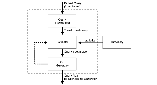
The input to the query transformer is a parsed query, which is represented by a set of query blocks. The query blocks are nested or interrelated to each other. The form of the query determines how the query blocks are interrelated to each other. The main objective of the query transformer is to determine if it is advantageous to change the form of the query so that it enables generation of a better query plan. Four different query transformation techniques are employed by the query transformer:
Any combination of these transformations can be applied to a given query.
Each view referenced in a query is expanded by the parser into a separate query block. The query block essentially represents the view definition, and therefore the result of a view. One option for the optimizer is to analyze the view query block separately and generate a view subplan. The optimizer then processes the rest of the query by using the view subplan in the generation of an overall query plan. This technique usually leads to a suboptimal query plan, because the view is optimized separately from rest of the query.
The query transformer then removes the potentially suboptimal plan by merging the view query block into the query block that contains the view. Most types of views are merged. When a view is merged, the query block representing the view is merged into the containing query block. Generating a subplan is no longer necessary, because the view query block is eliminated.
For those views that are not merged, the query transformer can push the relevant predicates from the containing query block into the view query block. This technique improves the subplan of the nonmerged view, because the pushed-in predicates can be used either to access indexes or to act as filters.
Like a view, a subquery is represented by a separate query block. Because a subquery is nested within the main query or another subquery, the plan generator is constrained in trying out different possible plans before it finds a plan with the lowest cost. For this reason, the query plan produced might not be the optimal one. The restrictions due to the nesting of subqueries can be removed by unnesting the subqueries and converting them into joins. Most subqueries are unnested by the query transformer. For those subqueries that are not unnested, separate subplans are generated. To improve execution speed of the overall query plan, the subplans are ordered in an efficient manner.
A materialized view is like a query with a result that is materialized and stored in a table. When a user query is found compatible with the query associated with a materialized view, the user query can be rewritten in terms of the materialized view. This technique improves the execution of the user query, because most of the query result has been precomputed. The query transformer looks for any materialized views that are compatible with the user query and selects one or more materialized views to rewrite the user query. The use of materialized views to rewrite a query is cost-based. That is, the query is not rewritten if the plan generated without the materialized views has a lower cost than the plan generated with the materialized views.
See Also:
|
The estimator generates three different types of measures:
These measures are related to each other, and one is derived from another. The end goal of the estimator is to estimate the overall cost of a given plan. If statistics are available, then the estimator uses them to compute the measures. The statistics improve the degree of accuracy of the measures.
The first measure, selectivity, represents a fraction of rows from a row set. The row set can be a base table, a view, or the result of a join or a GROUP BY operator. The selectivity is tied to a query predicate, such as last_name = 'Smith', or a combination of predicates, such as last_name = 'Smith' AND job_type = 'Clerk'. A predicate acts as a filter that filters a certain number of rows from a row set. Therefore, the selectivity of a predicate indicates how many rows from a row set will pass the predicate test. Selectivity lies in a value range from 0.0 to 1.0. A selectivity of 0.0 means that no rows will be selected from a row set, and a selectivity of 1.0 means that all rows will be selected.
The estimator uses an internal default value for selectivity, if no statistics are available. Different internal defaults are used, depending on the predicate type. For example, the internal default for an equality predicate (last_name = 'Smith') is lower than the internal default for a range predicate (last_name > 'Smith'). The estimator makes this assumption because an equality predicate is expected to return a smaller fraction of rows than a range predicate.
When statistics are available, the estimator uses them to estimate selectivity. For example, for an equality predicate (last_name = 'Smith'), selectivity is set to the reciprocal of the number n of distinct values of last_name, because the query selects rows that all contain one out of n distinct values. If a histogram is available on the last_name column, then the estimator uses it instead of the number of distinct values. The histogram captures the distribution of different values in a column, so it yields better selectivity estimates. Having histograms on columns that contain skewed data (in other words, values with large variations in number of duplicates) greatly helps the CBO generate good selectivity estimates.
Cardinality represents the number of rows in a row set. Here, the row set can be a base table, a view, or the result of a join or GROUP BY operator.
Base cardinality is the number of rows in a base table. The base cardinality can be captured by analyzing the table. If table statistics are not available, then the estimator uses the number of extents occupied by the table to estimate the base cardinality.
Effective cardinality is the number of rows that are selected from a base table. The effective cardinality depends on the predicates specified on different columns of a base table, with each predicate acting as a successive filter on the rows of the base table. The effective cardinality is computed as the product of the base cardinality and combined selectivity of all predicates specified on a table. When there is no predicate on a table, its effective cardinality equals its base cardinality.
Join cardinality is the number of rows produced when two row sets are joined together. A join is a Cartesian product of two row sets, with the join predicate applied as a filter to the result. Therefore, the join cardinality is the product of the cardinalities of two row sets, multiplied by the selectivity of the join predicate.
Distinct cardinality is the number of distinct values in a column of a row set. The distinct cardinality of a row set is based on the data in the column. For example, in a row set of 100 rows, if distinct column values are found in 20 rows, then the distinct cardinality is 20.
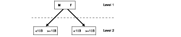
Group cardinality is the number of rows produced from a row set after the GROUP BY operator is applied. The effect of the GROUP BY operator is to decrease the number of rows in a row set. The group cardinality depends on the distinct cardinality of each of the grouping columns and on the number of rows in the row set. For an illustration of group cardinality, see Example 1-2.
If a row set of 100 rows is grouped by colx, which has a distinct cardinality of 30, then the group cardinality is 30.
However, suppose the same row set of 100 rows is grouped by colx and coly, which have distinct cardinalities of 30 and 60, respectively. In this case, the group cardinality lies between the maximum of the distinct cardinalities of colx and coly, and the lower of the product of the distinct cardinalities of colx and coly, and the number of rows in the row set.
Group cardinality in this example can be represented by the following formula:
group cardinality lies between max ( dist. card. colx
                                   , dist. card. coly )
                               and min ( (dist. card. colx * dist. card. coly)
                                   , num rows in row set )
Substituting the numbers from the example, the group cardinality is between the maximum of (30 and 60) and the minimum of (30*60 and 100). In other words, the group cardinality is between 60 and 100.
The cost represents units of work or resource used. The CBO uses disk I/O, CPU usage, and memory usage as units of work. So, the cost used by the CBO represents an estimate of the number of disk I/Os and the amount of CPU and memory used in performing an operation. The operation can be scanning a table, accessing rows from a table by using an index, joining two tables together, or sorting a row set. The cost of a query plan is the number of work units that are expected to be incurred when the query is executed and its result produced.
The access path represents the number of units of work required to get data from a base table. The access path can be a table scan, a fast full index scan, or an index scan. During table scan or fast full index scan, multiple blocks are read from the disk in a single I/O operation. Therefore, the cost of a table scan or a fast full index scan depends on the number of blocks to be scanned and the multiblock read count value. The cost of an index scan depends on the levels in the B-tree, the number of index leaf blocks to be scanned, and the number of rows to be fetched using the rowid in the index keys. The cost of fetching rows using rowids depends on the index clustering factor.
Although the clustering factor is a property of the index, the clustering factor actually relates to the spread of similar indexed column values within data blocks in the table. A lower clustering factor indicates that the individual rows are concentrated within fewer blocks in the table. Conversely, a high clustering factor indicates that the individual rows are scattered more randomly across blocks in the table. Therefore, a high clustering factor means that it costs more to use a range scan to fetch rows by rowid, because more blocks in the table need to be visited to return the data. Example 1-3 shows how the clustering factor can affect cost.
Assume the following situation:
col1 (in tab1).c1 column currently stores the values A, B, and C.Case 1: The index clustering factor is low for the rows as they are arranged in the following diagram.
                 Block 1       Block 2        Block 3
                 -------       -------        --------
                 A  A  A       B  B  B        C  C  C
This is because the rows that have the same indexed column values for c1 are located within the same physical blocks in the table. The cost of using a range scan to return all of the rows that have the value A is low, because only one block in the table needs to be read.
Case 2: If the same rows in the table are rearranged so that the index values are scattered across the table blocks (rather than colocated), then the index clustering factor is higher.
                 Block 1       Block 2        Block 3
                 -------       -------        --------
                 A  B  C       A  B  C        A  B  C
This is because all three blocks in the table must be read in order to retrieve all rows with the value A in col1.
The join cost represents the combination of the individual access costs of the two row sets being joined. In a join, one row set is called inner, and the other is called outer.
cost = outer access cost + (inner access cost * outer cardinality)
cost = outer access cost + inner access cost + sort costs (if sort is used)
Each row from the outer row set is hashed to probe matching rows in the hash partition. The next portion of the inner row set is then hashed into memory, followed by a probe from the outer row set. This process is repeated until all partitions of the inner row set are exhausted.
cost = (outer access cost * # of hash partitions) + inner access cost
| See Also:
"Understanding Joins" for more information on joins |
The main function of the plan generator is to try out different possible plans for a given query and pick the one that has the lowest cost. Many different plans are possible because of the various combinations of different access paths, join methods, and join orders that can be used to access and process data in different ways and produce the same result.
A join order is the order in which different join items (such as tables) are accessed and joined together. For example, in a join order of t1, t2, and t3, table t1 is accessed first. Next, t2 is accessed, and its data is joined to t1 data to produce a join of t1 and t2. Finally, t3 is accessed, and its data is joined to the result of the join between t1 and t2.
The plan for a query is established by first generating subplans for each of the nested subqueries and nonmerged views. Each nested subquery or nonmerged view is represented by a separate query block. The query blocks are optimized separately in a bottom-up order. That is, the innermost query block is optimized first, and a subplan is generated for it. The outermost query block, which represents the entire query, is optimized last.
The plan generator explores various plans for a query block by trying out different access paths, join methods, and join orders. The number of possible plans for a query block is proportional to the number of join items in the FROM clause. This number rises exponentially with the number of join items.
The plan generator uses an internal cutoff to reduce the number of plans it tries when finding the one with the lowest cost. The cutoff is based on the cost of the current best plan. If the current best cost is large, then the plan generator tries harder (in other words, explores more alternate plans) to find a better plan with lower cost. If the current best cost is small, then the plan generator ends the search swiftly, because further cost improvement will not be significant.
The cutoff works well if the plan generator starts with an initial join order that produces a plan with cost close to optimal. Finding a good initial join order is a difficult problem. The plan generator uses a simple heuristic for the initial join order. It orders the join items by their effective cardinalities. The join item with the smallest effective cardinality goes first, and the join item with the largest effective cardinality goes last.
Access paths are ways in which data is retrieved from the database. Any row in any table can be located and retrieved by one of the following methods:
In general, index access paths should be used for statements that retrieve a small subset of table rows, while full scans are more efficient when accessing a large portion of the table. Online transaction processing (OLTP) applications, which consist of short-running SQL statements with high selectivity, often are characterized by the use of index access paths. Decision support systems, on the other hand, tend to use partitioned tables and perform full scans of the relevant partitions.
This section describes the following data access paths:
During a full table scan, all blocks in the table that are under the high water mark are scanned. Each row is examined to determine whether it satisfies the statement's WHERE clause.
When Oracle performs a full table scan, the blocks are read sequentially. Because the blocks are adjacent, I/O calls larger than a single block can be used to speed up the process. The size of the read calls range from one block to the number of blocks indicated by the initialization parameter DB_FILE_MULTIBLOCK_READ_COUNT. Using multiblock reads means a full table scan can be performed very efficiently. Each block is read only once.
In Example 1-4, suppose you need to do a case-independent search for a name on a table containing all employees.
SELECT last_name, first_name
  FROM employees
 WHERE UPPER(last_name) LIKE :b1

Plan
-------------------------------------------------
SELECT STATEMENT
 TABLE ACCESS FULL EMPLOYEES
Although the table might have several thousand employees, the number of rows for a given name ranges from 1 to 20. It might be better to use an index to access the desired rows, and there is an index on last_name in employees.
However, the optimizer is unable to use the index because there is a function on the indexed column. With no access path, the optimizer uses a full table scan. If you need to use the index for case-independent searches, then either do not permit mixed-case data in the search columns or else do not allow function-based indexes to be created on search columns.
The optimizer uses a full table scan in any of the following cases:
If the query is unable to use any existing indexes, then it uses a full table scan.
If the optimizer thinks that the query will access most of the blocks in the table, then it uses a full table scan, even though indexes might be available.
If a table contains less than DB_FILE_MULTIBLOCK_READ_COUNT blocks under the high water mark, which can be read in a single I/O call, then a full table scan might be cheaper than an index range scan, regardless of the fraction of tables being accessed or indexes present.
If the table has not been analyzed since it was created, and if it has less than DB_FILE_MULTIBLOCK_READ_COUNT blocks under the high water mark, then the optimizer thinks that the table is small and uses a full table scan. Look at the LAST_ANALYZED and BLOCKS columns in the ALL_TABLES table to see what the statistics reflect.
A high degree of parallelism for a table skews the optimizer toward full table scans over range scans. Examine the DEGREE column in ALL_TABLES for the table to determine the degree of parallelism.
Use the hint FULL(table alias).
SELECT last_name, first_name
  FROM employees
 WHERE last_name LIKE :b1;

Plan
-------------------------------------------------
SELECT STATEMENT
 TABLE ACCESS BY INDEX ROWID EMPLOYEES
  INDEX RANGE SCAN EMPLOYEES
SELECT /*+ FULL(e) */ last_name, first_name FROM employees e WHERE last_name LIKE :b1;Plan-------------------------------------------------SELECT STATEMENTTABLE ACCESS FULL EMPLOYEES
Full table scans are cheaper than index range scans when accessing a large fraction of the blocks in a table. This is because full table scans can use larger I/O calls, and making fewer large I/O calls is cheaper than making many smaller calls.
The elapsed time for an I/O call consists of two components:
In a typical I/O operation, setup costs consume most of the time. Data transfer time for an 8-K buffer is less than 1 msec (out of the total time of 10 msec). This means that you can transfer 128 KB in about 20 msec with a single 128 KB call, as opposed to needing 160 msec with sixteen 8-KB calls. Example 1-7 illustrates a typical case.
Consider a case in which 20% of the blocks in a 10,000-block table are accessed. The following are true:
DB_FILE_MULTIBLOCK_READ_COUNT = 16DB_BLOCK_SIZE = 8 KAssume that each 8 K I/O takes 10 msec, and about 20 seconds are spent doing single block I/O for the table blocks. This does not include the additional time to perform the index block I/O. Assuming that each 128 K I/O takes 20 msec, about 12.5 seconds are spent waiting for the data blocks, with no wait required for any index blocks.
The total time changes when CPU numbers are added in for crunching all the rows for a full table scan and for processing the index access in the range scan. But, the full table scan comes out faster with such a large fraction of blocks being accessed.
Oracle does I/O by blocks. Therefore, the optimizer's decision to use full table scans is influenced by the percentage of blocks accessed, not rows. This is called the index clustering factor. If blocks contain single rows, then rows accessed and blocks accessed are the same.
However, most tables have multiple rows in each block. Consequently, the desired number of rows could be clustered together in a few blocks, or they could be spread out over a larger number of blocks.
Consider a case where each block has 100 rows, but on an average only 5 rows for each block meet the query condition. A query accessing 2% of the rows might need 40% of the blocks.
| See Also:
"Estimator" for more information on the index clustering factor |
The data dictionary keeps track of the blocks that have been populated with rows. The high water mark is used as the end marker during a full table scan. The high water mark is stored in DBA_TABLES.BLOCKS. It is reset when the table is dropped or truncated.
For example, consider a table that had a large number of rows in the past. Most of the rows have been deleted, and now most of the blocks under the high water mark are empty. A full table scan on this table exhibits poor performance because all the blocks under the high water mark are scanned.
When a full table scan is required, response time can be improved by using multiple parallel execution servers for scanning the table. Parallel queries are used generally in low-concurrency data warehousing environments, because of the potential resource usage.
A sample table scan retrieves a random sample of data from a table. This access path is used when a statement's FROM clause includes the SAMPLE clause or the SAMPLE BLOCK clause. To perform a sample table scan when sampling by rows (the SAMPLE clause), Oracle reads a specified percentage of rows in the table. To perform a sample table scan when sampling by blocks (the SAMPLE BLOCK clause), Oracle reads a specified percentage of table blocks.
Oracle does not support sample table scans when the query involves a join or a remote table. However, you can perform an equivalent operation by using a CREATE TABLE AS SELECT query to materialize a sample of an underlying table. You then rewrite the original query to refer to the newly created table sample. Additional queries can be written to materialize samples for other tables. Sample table scans require the CBO.
Example 1-8 uses a sample table scan to access 1% of the employees table, sampling by blocks.
SELECT *
    FROM employees SAMPLE BLOCK (1);
The EXPLAIN PLAN output for this statement might look like this:
OPERATION                 OPTIONS        OBJECT_NAME
-----------------------------------------------------
SELECT STATEMENT
  TABLE ACCESS            SAMPLE         EMPLOYEES
The rowid of a row specifies the datafile and data block containing the row and the location of the row in that block. Locating a row by its rowid is the fastest way for Oracle to find a single row.
To access a table by rowid, Oracle first obtains the rowids of the selected rows, either from the statement's WHERE clause or through an index scan of one or more of the table's indexes. Oracle then locates each selected row in the table based on its rowid.
In Example 1-9, an index range scan is performed. The rowids retrieved are used to return the row data.
SELECT last_name, first_name
  FROM employees
 WHERE last_name = :b1;

Plan
-------------------------------------------------
SELECT STATEMENT
 TABLE ACCESS BY INDEX ROWID EMPLOYEES
  INDEX RANGE SCAN EMPLOYEES
This is generally the second step after retrieving the rowid from an index. The table access might be required for any columns in the statement not present in the index.
Access by rowid does not need to follow every index scan. If the index contains all the columns needed for the statement, then table access by rowid might not occur.
|
Note: Rowids are an internal Oracle representation of where data is stored. They can change between versions. Accessing data based on position is not recommended, because rows can move around due to row migration and chaining and also after export and import. Foreign keys should be based on primary keys. For more information on rowids, see Oracle9i Application Developer's Guide - Fundamentals. |
An index scan retrieves data from an index based on the value of one or more columns in the index. To perform an index scan, Oracle searches the index for the indexed column values accessed by the statement. If the statement accesses only columns of the index, then Oracle reads the indexed column values directly from the index, rather than from the table.
The index contains not only the indexed value, but also the rowids of rows in the table having that value. Therefore, if the statement accesses other columns in addition to the indexed columns, then Oracle can find the rows in the table by using either a table access by rowid or a cluster scan.
An index scan can be one of the following types:
This scan returns, at most, a single rowid. Oracle performs a unique scan if a statement contains a UNIQUE or a PRIMARY KEY constraint that guarantees that only a single row is accessed.
Example 1-10 queries the orders table orders for a given order (order_id).
SELECT <attribute2>
  FROM orders
 WHERE order_id = :b1
   AND order_mode = :b2;

Plan
-------------------------------------------------
SELECT STATEMENT
 TABLE ACCESS BY ROWID OF ORDERS
  INDEX UNIQUE SCAN  OF ORDER_ID
This access path is used when all columns of a unique (B-tree) index are specified with equality conditions.
None of the statements in Example 1-11 use a UNIQUE scan, because the complete unique key is not being used in the equality condition.
SELECT <attribute2>
  FROM orders
 WHERE order_id = :b1
   AND order_mode > 0;

Plan
-------------------------------------------------
SELECT STATEMENT
 TABLE ACCESS BY ROWID  OF ORDERS
  INDEX RANGE SCAN  OF ORDER_ID
| See Also:
Oracle9i Database Concepts for more details on index structures and for detailed information on how a B-tree is searched |
In general, you should not need to use a hint to do a unique scan. There might be cases where the table is across a database link and being accessed from a local table, or where the table is small enough for the optimizer to prefer a full table scan.
The hint INDEX(alias index_name) specifies the index to use, but not an access path (range scan or unique scan).
An index range scan is a common operation for accessing selective data. It can be bounded (bounded on both sides) or unbounded (on one or both sides). Data is returned in the ascending order of index columns. Multiple rows with identical values are sorted in ascending order by rowid.
If data must be sorted by order, then use the ORDER BY clause, and do not rely on an index. If an index can be used to satisfy an ORDER BY clause, then the optimizer uses this option and avoids a sort.
In Example 1-12, the order has been imported from a legacy system, and you are querying the order by the number in the legacy system.
SELECT <attribute2>, order_id
  FROM orders
 WHERE <original_system_reference> = :b1;

Plan
-------------------------------------------------
SELECT STATEMENT
 TABLE ACCESS BY ROWID  OF ORDERS
  INDEX RANGE SCAN  OF <original_system_reference>
This should be a highly selective query, and you should see the query using the index on the column to retrieve the desired rows. The data returned is sorted in ascending order by the rowids for the <original_system_reference>. Because the index column <original_system_reference> is identical for the selected rows here, the data is sorted by rowid.
The optimizer uses a range scan when it finds one or more leading columns of an index specified in conditions, such as the following:
col1 = :b1col1 < :b1col1 > :b1AND combination of the preceding conditions for leading columns in the indexcol1 like '%ASD' Wild-card searches should not be in a leading position. The condition col1 like '%ASD' does not result in a range scan..Range scans can use unique or nonunique indexes. Range scans avoid sorting when index columns constitute the ORDER BY/GROUP BY clause.
A hint might be required if the optimizer chooses some other index or uses a full table scan. The hint INDEX(table_alias index_name) specifies the index to use.
In Example 1-13, the column S2 has a skewed distribution:
    S2       Rows     Blocks
------ ---------- ----------
     0        769        347
     4       1460        881
     5          5          4
     8        816        590
    18  1,028,946    343,043
The column has histograms, so the optimizer knows about the distribution. However, with a bind variable, the optimizer does not know the value and could choose a full table scan. Therefore, you have two options:
SELECT l.line_item_id, l.<revenue_amount>
  FROM order_items l
 WHERE l.s2 = :b1;

Plan
-------------------------------------------------
SELECT STATEMENT
 TABLE ACCESS FULL ORDER_ITEMS
SELECT l.line_item_id, l.<revenue_amount>
  FROM order_items l
 WHERE l.s2 = 4;

Plan
-------------------------------------------------
SELECT STATEMENT
 TABLE ACCESS BY INDEX ROWID ORDER_ITEMS
  INDEX RANGE SCAN ORDER_ITEMS_N7
SELECT /*+ INDEX(l order_items_n7) */ l.line_item_id, l.<revenue_amount>
  FROM order_items l
 WHERE l.s2 = :b1;

Plan
-------------------------------------------------
SELECT STATEMENT
 TABLE ACCESS BY INDEX ROWID ORDER_ITEMS
  INDEX RANGE SCAN ORDER_ITEMS_N7
An index range scan descending is identical to an index range scan, except that the data is returned in descending order. (Indexes, by default, are stored in ascending order.) Usually, this scan is used when ordering data in a descending order to return the most recent data first, or when seeking a value less than a specified value.
Example 1-17 uses a two-column unique index on order_id, order_mode.
SELECT <attribute2>, order_id
  FROM orders a
 WHERE order_id = :b1
 ORDER BY order_id DESC;

Plan
-------------------------------------------------
SELECT STATEMENT
 TABLE ACCESS BY ROWID  OF ORDERS
  INDEX RANGE SCAN DESCENDING ORDER_ID
The data is sorted in descending order by the order_id, order_mode, rowid of the selected rows. However, because there is only one row for each order_id, order_mode (orders_u2 is a unique index on the two columns), the rows are sorted by order_id, order_mode.
Example 1-18 uses a single-column index on <purchase_order_num>. The data is retrieved in descending order by <purchase_order_num>, rowid.
SELECT <attribute2>, order_id
  FROM orders a
 WHERE <purchase_order_num> BETWEEN :b1 AND :b2
 ORDER BY <purchase_order_num> DESC;

Plan
-------------------------------------------------
SELECT STATEMENT
 TABLE ACCESS BY INDEX ROWID ORDERS
  INDEX RANGE SCAN DESCENDING ORDER_ID
The optimizer uses index range scan descending when an order by descending clause can be satisfied by an index.
The hint INDEX_DESC(table_alias index_name) is used for this access path.
Initial Query
SELECT a.<original_system_reference>, a.<original_system_code>, a.order_id FROM orders a WHERE a.<original_system_reference>= :b1; Plan ------------------------------------------------- SELECT STATEMENT TABLE ACCESS BY INDEX ROWID ORDERS INDEX RANGE SCAN <original_system_reference>
Query Using INDEX_DESC Hint
SELECT /*+INDEX_DESC(a<original_system_reference>) */ a.<original_system_reference>, a.<original_system_code>, a.order_id FROM orders a WHERE a.<original_system_reference>= :b1;
The data with this hint is sorted in descending order by <original_system_reference>, <original_system_code>, rowid.
Plan
-------------------------------------------------
SELECT STATEMENT
 TABLE ACCESS BY INDEX ROWID ORDERS
  INDEX RANGE SCAN DESCENDING <original_system_reference>
Alternate Query Using INDEX_DESC Hint
SELECT /*+INDEX_DESC(a orders_n9) */
       a.<original_system_reference>, a.<original_system_code>, a.order_id
  FROM orders a
 WHERE a.original_system_reference = :b1;
The data with this hint is sorted in descending order by <original_system_reference>, rowid.
Plan
-------------------------------------------------
SELECT STATEMENT
 TABLE ACCESS BY INDEX ROWID ORDERS
  INDEX RANGE SCAN DESCENDING <original_system_reference>
Index skip scans improve index scans by nonprefix columns. Often, scanning index blocks is faster than scanning table data blocks.
Skip scanning lets a composite index be split logically into smaller subindexes. In skip scanning, the initial column of the composite index is not specified in the query. In other words, it is "skipped."
The number of logical subindexes is determined by the number of distinct values in the initial column. Skip scanning is advantageous if there are few distinct values in the leading column of the composite index and many distinct values in the nonleading key of the index.
Consider, for example, a table employees (sex, employee_id, address) with a composite index on (sex, employee_id). Splitting this composite index would result in two logical subindexes, one for M and one for F.
For this example, suppose you have the following index data:
 (`F',98)
 (`F',100)
 (`F',102)
 (`F',104)
 (`M',101)
 (`M',103)
 (`M',105)
The index is split logically into the following two subindexes:
`F'.`M'.
The column sex is skipped in the following query:
SELECT *
FROM employees
WHERE employee_id = 101;
A complete scan of the index is not performed, but the subindex with the value `F' is searched first, followed by a search of the subindex with the value `M'.
A full scan is available if a predicate references one of the columns in the index. The predicate does not need to be an index driver. A full scan is also available when there is no predicate, if both the following conditions are met:
A full scan can be used to eliminate a sort operation, because the data is ordered by the index key. It reads the blocks singly.
Fast full index scans are an alternative to a full table scan when the index contains all the columns that are needed for the query, and at least one column in the index key has the NOT NULL constraint. A fast full scan accesses the data in the index itself, without accessing the table. It cannot be used to eliminate a sort operation, because the data is not ordered by the index key. It reads the entire index using multiblock reads (unlike a full index scan) and can be parallelized.
Fast full scan is available only with the CBO. You can specify it with the initialization parameter OPTIMIZER_FEATURES_ENABLE or the INDEX_FFS hint. Fast full index scans cannot be performed against bitmap indexes.
A fast full scan is faster than a normal full index scan in that it can use multiblock I/O and can be parallelized just like a table scan. Example 1-21 illustrates this feature.
SELECT COUNT(*)
FROM t1, t2
WHERE t1.c1 > 50
     AND t1.c2 = t2.c1;

Plan
-------------------------------------------------
SELECT STATEMENT
     SORT AGGREGATE
          HASH JOIN
               TABLE ACCESS t1 FULL
               INDEX t2_c1_idx FAST FULL SCAN
Because index t2_c1_idx contains all the columns needed from table t2, the optimizer uses a fast full index scan on that index.
Fast full index scans have the following restrictions:
NOT NULL constraint.The fast full scan has a special index hint, INDEX_FFS, which has the same format and arguments as the regular INDEX hint.
| See Also:
Chapter 5, "Optimizer Hints" for detailed information on the |
An index join is a hash join of several indexes that together contain all the table columns that are referenced in the query. If an index join is used, then no table access is needed, because all the relevant column values can be retrieved from the indexes. An index join cannot be used to eliminate a sort operation. The index join is available only with the CBO.
Example 1-22 uses an index join to access the employee_id and salary columns, both of which are indexed, in the employees table.
SELECT employee_id, salary
    FROM employees
    WHERE salary > 2000;

Plan
---------------------------------------------------------
OPERATION               OPTIONS          OBJECT_NAME
---------------------------------------------------------
SELECT STATEMENT
  VIEW                                   index$_join$_001
    HASH JOIN
      INDEX             RANGE SCAN       EMP_SALARY
      INDEX             FAST FULL SCAN   EMP_EMPLOYEE_ID
You can specify an index join with the initialization parameter OPTIMIZER_FEATURES_ENABLE or the INDEX_JOIN hint.
A bitmap join uses a bitmap for key values and a mapping function that converts each bit position to a rowid. Bitmaps can efficiently merge indexes that correspond to several conditions in a WHERE clause, using Boolean operations to resolve AND and OR conditions.
Bitmap access is available only with the CBO.
|
Note: Bitmap indexes and bitmap join indexes are available only if you have purchased the Oracle9i Enterprise Edition.. |
| See Also:
Oracle9i Data Warehousing Guide for more information about bitmap indexes |
A cluster scan is used to retrieve, from a table stored in an indexed cluster, all rows that have the same cluster key value. In an indexed cluster, all rows with the same cluster key value are stored in the same data block. To perform a cluster scan, Oracle first obtains the rowid of one of the selected rows by scanning the cluster index. Oracle then locates the rows based on this rowid.
A hash scan is used to locate rows in a hash cluster, based on a hash value. In a hash cluster, all rows with the same hash value are stored in the same data block. To perform a hash scan, Oracle first obtains the hash value by applying a hash function to a cluster key value specified by the statement. Oracle then scans the data blocks containing rows with that hash value.
The CBO chooses an access path based on the following factors:
To choose an access path, the optimizer first determines which access paths are available by examining the conditions in the statement's WHERE clause (and its FROM clause for the SAMPLE or SAMPLE BLOCK clause). The optimizer then generates a set of possible execution plans using available access paths and estimates the cost of each plan, using the statistics for the index, columns, and tables accessible to the statement. Finally, the optimizer chooses the execution plan with the lowest estimated cost.
The optimizer's choice among available access paths can be overridden with hints, except when the statement's FROM clause contains SAMPLE or SAMPLE BLOCK.
| See Also:
Chapter 5, "Optimizer Hints" for information about hints in SQL statements |
Example 1-23 illustrates how the optimizer chooses an access path.
The following query uses an equality condition in its WHERE clause to select all employees named Jackson:
SELECT *
  FROM employees
  WHERE last_name = 'JACKSON';
If the last_name column is a unique or primary key, then the optimizer determines that there is only one employee named Jackson, and the query returns only one row. In this case, the query is very selective, and the optimizer is most likely to access the table using a unique scan on the index that enforces the unique or primary key.
Consider again the query in the previous example. If the last_name column is not a unique or primary key, then the optimizer can use the following statistics to estimate the query's selectivity:
USER_TAB_COLUMNS.NUM_DISTINCT, which is the number of values for each column in the tableUSER_TABLES.NUM_ROWS, which is the number of rows in each tableBy dividing the number of rows in the employees table by the number of distinct values in the last_name column, the optimizer estimates what percentage of employees have the same name. By assuming that the last_name values are distributed uniformly, the optimizer uses this percentage as the estimated selectivity of the query.
The following query selects all employees with employee ID numbers less than 7500:
SELECT *
  FROM employees
  WHERE employee_id < 7500;
To estimate the selectivity of the query, the optimizer uses the boundary value of 7500 in the WHERE clause condition and the values of the HIGH_VALUE and LOW_VALUE statistics for the employee_id column, if available. These statistics can be found in the USER_TAB_COL_STATISTICS view (or the USER_TAB_COLUMNS view). The optimizer assumes that employee_id values are distributed evenly in the range between the lowest value and highest value. The optimizer then determines what percentage of this range is less than the value 7500 and uses this value as the estimated selectivity of the query.
The following query uses a bind variable rather than a literal value for the boundary value in the WHERE clause condition:
SELECT *
  FROM employees
  WHERE employee_id < :e1;
The optimizer does not know the value of the bind variable e1. Indeed, the value of e1 might be different each time the query is executed. For this reason, the optimizer cannot use the means described in the previous example to determine selectivity of this query. In this case, the optimizer heuristically guesses a small value for the selectivity, using an internal default value. The optimizer makes this assumption whenever a bind variable is used as a boundary value in a condition with one of the following operators: <, >, <=, or >=.
The optimizer's treatment of bind variables can cause it to choose different execution plans for SQL statements that differ only in the use of bind variables rather than constants. For example, the optimizer might choose different execution plans for an embedded SQL statement with a bind variable in an Oracle precompiler program and the same SQL statement with a constant in SQL*Plus.
The following query uses two bind variables as boundary values in the condition with the BETWEEN operator:
SELECT *
  FROM employees
  WHERE employee_id BETWEEN :low_e AND :high_e;
The optimizer rewrites the BETWEEN condition as the following two conditions:
employee_id >= :low_e
employee_id <= :high_e
The optimizer heuristically estimates a small selectivity (an internal default value) for indexed columns in order to favor the use of the index.
The following query uses the BETWEEN operator to select all employees with employee ID numbers between 7500 and 7800:
SELECT *
  FROM employees
  WHERE employee_id BETWEEN 7500 AND 7800;
To determine the selectivity of this query, the optimizer rewrites the WHERE clause condition into the following two conditions:
employee_id >= 7500
employee_id <= 7800
The optimizer estimates the individual selectivity of each condition, using the means described in Case 4. The optimizer then uses these selectivities (S1 and S2) and the absolute value function (ABS) to estimate the selectivity (S) of the BETWEEN condition, as follows:
S = ABS(S1 + S2 - 1)
Joins are statements that retrieve data from more than one table. A join is characterized by multiple tables in the FROM clause, and the relationship between the tables is defined through the existence of a join condition in the WHERE clause.
This section discusses how the Oracle optimizer executes SQL statements that contain joins, anti-joins, and semi-joins. It also describes how the optimizer can use bitmap indexes to execute star queries, which join a fact table to multiple dimension tables.
To choose an execution plan for a join statement, the optimizer must make these interrelated decisions:
As for simple statements, the optimizer must choose an access path to retrieve data from each table in the join statement.
To join each pair of row sources, Oracle must perform one of the following operations:
To execute a statement that joins more than two tables, Oracle joins two of the tables and then joins the resulting row source to the next table. This process is continued until all tables are joined into the result.
The optimizer estimates the cost of each join method and chooses the method with the least cost. If a join returns many rows, then the optimizer considers the following three factors:
cost = access cost of A + (access cost of B * number of rows from A)
cost = (access cost of A * number of hash partitions of B) + access cost of B
cost = access cost of A + access cost of B + (sort cost of A + sort cost of B)
When the data is presorted, the sort costs are both zero.
Nested loop joins are useful when small subsets of data are being joined and if the join condition is an efficient way of accessing the second table.
It is very important to ensure that the inner table is driven from (dependent on) the outer table. If the inner table's access path is independent of the outer table, then the same rows are retrieved for every iteration of the outer loop, degrading performance considerably. In such cases, hash joins joining the two independent row sources perform better.
A nested loop join involves the following steps:
NESTED LOOP
  <Outer Loop>
  <Inner Loop>
Consider the execution plan for the following query:
SELECT a.unit_price * a.quantity
  FROM order_items a,orders b
 WHERE b.customer_id = :b1
   AND a.order_id = b.order_id

Plan
-------------------------------------------------
SELECT STATEMENT
 NESTED LOOPS
  TABLE ACCESS BY INDEX ROWID ORDERS
   INDEX RANGE SCAN CUSTOMER_ID
  TABLE ACCESS BY INDEX ROWID ORDER_ITEMS
   INDEX RANGE SCAN ORDER_ID
In this execution plan, the outer loop and the equivalent statement are as follows:
TABLE ACCESS BY INDEX ROWID ORDERS
 INDEX RANGE SCAN CUSTOMER_ID

SELECT <some columns>
  FROM orders b
 WHERE b.customer_id = :b1
The execution plan shows the inner loop being iterated for every row fetched from the outer loop, as follows:
TABLE ACCESS BY INDEX ROWID ORDER_ITEMS
 INDEX RANGE SCAN ORDER_ID

SELECT <some columns>
  FROM order_items a
WHERE a.<order_id> = :b2
Therefore, the statement that retrieves the lines for a customer can be broken down into two loops:
The optimizer uses nested loop joins when joining small number of rows, with a good driving condition between the two tables. You drive from the outer loop to the inner loop, so the order of tables in the execution plan is important.
The outer loop is the driving row source. It produces a set of rows for driving the join condition. The row source can be a table accessed using an index scan or a full table scan. Also, the rows can be produced from any other operation. For example, the output from a nested loop join can be used as a row source for another nested loop join.
The inner loop is iterated for every row returned from the outer loop, ideally by an index scan. If the access path for the inner loop is not dependent on the outer loop, then you can end up with a Cartesian product; for every iteration of the outer loop, the inner loop produces the same set of rows. Therefore, you should use other join methods when two independent row sources are joined together.
If the optimizer is choosing to use some other join method, use the USE_NL(a b) hint, where a and b are the aliases of the tables being joined.
In Example 1-25, the data is small enough for the optimizer to prefer full table scans and use hash joins.
Initial Query
SELECT l.unit_price * l.quantity
  FROM order_items l, orders h
 WHERE h.customer_id = :b1
   AND l.order_id = h.order_id;

Plan
-------------------------------------------------
SELECT STATEMENT
 HASH JOIN
  TABLE ACCESS FULL ORDERS
  TABLE ACCESS FULL ORDER_ITEMS
Query Using Nested Loop Join Hint
The following example shows a hint that changes the join method to nested loop. In this statement, orders is accessed through a full table scan and the filter condition customer_id = :b1 is applied to every row. For every row that meets the filter condition, order_items is accessed through the index order_id.
SELECT /*+ USE_NL(l h) */ l.unit_price * l.quantity
  FROM order_items l, orders h
 WHERE h.customer_id = :b1
   AND l.order_id = h.order_id;

Plan
-------------------------------------------------
SELECT STATEMENT
 NESTED LOOPS
  TABLE ACCESS FULL ORDERS
  TABLE ACCESS BY INDEX ROWID ORDER_ITEMS
   INDEX RANGE SCAN ORDER_ID
Avoiding a Full Table Scan
Adding another hint here avoids the full table scan on orders, resulting in an execution plan similar to one used on larger systems (even though it might not be particularly efficient here).
SELECT /*+ USE_NL(l h) INDEX(h orders_n1) */ l.unit_price * l.quantity
  FROM order_items l, orders h
 WHERE h.customer_id = :b1
   AND l.order_id = h.order_id;

Plan
-------------------------------------------------
SELECT STATEMENT
 NESTED LOOPS
  TABLE ACCESS BY INDEX ROWID ORDERS
   INDEX RANGE SCAN CUSTOMER_ID
  TABLE ACCESS BY INDEX ROWID ORDER_ITEMS
   INDEX RANGE SCAN ORDER_ID
The outer loop of a nested loop can be a nested loop itself. You can nest two or more outer loops together to join as many tables as needed. Each loop is a data access method, as follows:
SELECT STATEMENT
 NESTED LOOP 3
  NESTED LOOP 2          (OUTER LOOP 3.1)
   NESTED LOOP 1         (OUTER LOOP 2.1)
    OUTER LOOP 1.1     - #1
    INNER LOOP 1.2     - #2
   INNER LOOP 2.2      - #3
  INNER LOOP 3.2       - #4
This operation is used when an outer join is used between two tables. The outer join returns the outer (preserved) table rows, even when there are no corresponding rows in the inner (optional) table.
In a regular outer join, the optimizer chooses the order of tables (driving and driven) based on the cost. However, in a nested loop outer join, the order of tables is determined by the join condition. The outer table (with rows that are being preserved) is used to drive to the inner table.
In Example 1-26, all the customers created in the last 30 days are queried to see how active they are. An outer join is needed so that you don't miss the customers who do not have any orders.
SELECT cust_last_name, 86(nvl2(h.customer_id,0,1)) "Count"
  FROM customers c, orders h
 WHERE c.<creation_date> > SYSDATE - 30
   AND c.customer_id = h.customer_id(+)
 GROUP BY cust_last_name;

Plan
--------------------------------------------------
SELECT STATEMENT
 SORT GROUP BY
  NESTED LOOPS OUTER
   TABLE ACCESS BY INDEX ROWID CUSTOMERS
    INDEX RANGE SCAN <creation_date>
   INDEX RANGE SCAN CUSTOMER_ID
In this case, the outer join condition is the following:
customers.customer_id = orders.customer_id(+)
In this outer join condition,
customers.orders.customers rows, including those rows without a corresponding row in orders.customers to orders.The optimizer uses nested loop joins to process an outer join in the following circumstances:
To have the optimizer to use a nested loop for a join, use the hint USE_NL.
Hash joins are used for joining large data sets. The optimizer uses the smaller of two tables or data sources to build a hash table on the join key in memory. It then scans the larger table, probing the hash table to find the joined rows.
This method is best used when the smaller table fits in available memory. The cost is then limited to a single read pass over the data for the two tables.
However, if the hash table grows too big to fit into the memory, then the optimizer breaks it up into different partitions. As the partitions exceed allocated memory, parts are written to temporary segments on disk. Larger temporary extent sizes lead to improved I/O when writing the partitions to disk; the recommended temporary extent is about 1 MB. Temporary extent size is specified by INITIAL and NEXT for permanent tablespaces and by UNIFORM SIZE for temporary tablespaces.
After the hash table is complete, the following processes occur:
When the hash table build is complete, it is possible that an entire hash table partition is resident in memory. Then, you do not need to build the corresponding partition for the second (larger) table. When that table is scanned, rows that hash to the resident hash table partition can be joined and returned immediately.
Each hash table partition is then read into memory, and the following processes occur:
This process is repeated for the rest of the partitions. The cost can increase to two read passes over the data and one write pass over the data.
If the hash table does not fit in the memory, it is possible that parts of it may need to be swapped in and out, depending on the rows retrieved from the second table. Performance for this scenario can be extremely poor.
The optimizer uses a hash join to join two tables if they are joined using an equijoin and if either of the following conditions are true:
In Example 1-27, the table orders is used to build the hash table, and order_items is the larger table, which is scanned later.
SELECT h.customer_id, l.unit_price * l.quantity
  FROM orders h ,order_items l
 WHERE l.order_id = h.order_id

Plan
-------------------------------------------------
SELECT STATEMENT
 HASH JOIN
  TABLE ACCESS FULL ORDERS
  TABLE ACCESS FULL ORDER_ITEMS
Apply the USE_HASH hint to advise the optimizer to use a hash join when joining two tables together. Investigate the values for the parameters HASH_AREA_SIZE and HASH_JOIN_ENABLED, if you are having trouble getting the optimizer to use hash joins.
USE_HASH HintInitial Query
SELECT l.<promise_date>,l.product_id, SUM(l2.quantity)
  FROM order_items l, order_items l2
 WHERE l.product_id = l2.product_id
   AND l.warehouse_id = l2.warehouse_id
   AND l2.<promise_date> < l.<promise_date>
GROUP BY l.product_id, l.<promise_date>, l.order_id

Plan
--------------------------------------------------
SELECT STATEMENT
 SORT GROUP BY
  MERGE JOIN
   SORT JOIN
    TABLE ACCESS FULL ORDER_ITEMS
   FILTER
    SORT JOIN
     TABLE ACCESS FULL ORDER_ITEMS
Query Using Hint
SELECT /*+USE_HASH(l l2) */ l.<promise_date>,l.product_id, SUM(l2.quantity)
  FROM order_items l, order_items l2
 WHERE l.product_id = l2.product_id
   AND l.warehouse_id = l2.warehouse_id
   AND l2.<promise_date> < l.<promise_date>
GROUP BY l.product_id, l.<promise_date>, l.order_id

Plan
--------------------------------------------------
SELECT STATEMENT
 SORT GROUP BY
  HASH JOIN
   TABLE ACCESS FULL ORDER_ITEMS
   TABLE ACCESS FULL ORDER_ITEMS
This operation is used for outer joins where the optimizer decides that the amount of data is large enough to warrant a hash join, or it is unable to drive from the outer table to the inner table.
Like an outer join, the order of tables is not determined by the cost, but by the join condition. The outer table (with preserved rows) is used to build the hash table, and the inner table is used to probe the hash table.
Example 1-29 shows a typical hash join outer join query.
SELECT cust_last_name
  FROM customers c, orders h
 WHERE c.<creation_date> < SYSDATE - 365
   AND h.customer_id(+) = c.customer_id
   AND h.customer_id IS NULL;

Plan
--------------------------------------------------
SELECT STATEMENT
 FILTER
  HASH JOIN OUTER
   TABLE ACCESS BY INDEX ROWID CUSTOMERS
    INDEX RANGE SCAN <creation_date>
   INDEX FAST FULL SCAN CUSTOMER_ID
The query looks for inactive customers (more than a year old, with no orders). An outer join returns NULL for the inner table columns along with the outer (preserved) table rows when it does not find any corresponding rows in the inner table. This operation finds all the customers rows that do not have any orders rows.
In this case, the outer join condition is the following:
customers.customer_id = orders.customer_id(+)
The components of this condition represent the following:
customers.orders.customers rows, including those rows without a corresponding row in orders.customers.orders.You could use a NOT EXISTS subquery to return the rows; however, because you are querying all the rows in the table, the hash join performs better (unless the NOT EXISTS subquery is not nested).
The optimizer uses hash joins for processing an outer join if the data volume is high enough to make the hash join method efficient or if it is not possible to drive from the outer table to inner table.
In Example 1-30, the outer join is to a multitable view. The optimizer cannot drive into the view like in a normal join or push the predicates, so it builds the entire row set of the view.
SELECT c.cust_last_name, sum(<revenue>)
  FROM customers c, orders h
 WHERE c.<creation_date> > sysdate - 30
   AND h.customer_id(+) = c.customer_id
 GROUP BY c.cust_last_name;

Plan
--------------------------------------------------
SELECT STATEMENT
 SORT GROUP BY
  HASH JOIN OUTER
   TABLE ACCESS BY INDEX ROWID CUSTOMERS
    INDEX RANGE SCAN <creation_date>
   VIEW  ORDERS
    SORT GROUP BY
     HASH JOIN
      TABLE ACCESS FULL ORDERS
      TABLE ACCESS FULL ORDER_ITEMS
The view definition us as follows:
CREATE OR REPLACE view orders AS
SELECT h.order_id, SUM(l.<revenue_amount>) <revenue>, h.order_id, h.customer_id
  FROM orders h, order_items l
 WHERE h.order_id = l.order_id
 GROUP BY h.order_id, h.order_id, h.customer_id;
To use a hash join for an outer join, apply the hint USE_HASH.
Sort merge joins can be used to join rows from two independent sources. Hash joins generally perform better than sort merge joins. On the other hand, sort merge joins can perform better than hash joins if both of the following conditions exist:
However, if a sort merge join involves choosing a slower access method (an index scan as opposed to a full table scan), then the benefit of using a sort merge might be lost.
Sort merge joins are useful when the join condition between two tables is an inequality condition (but not a nonequality) like <, <=, >, or >=. Sort merge joins perform better than nested loop joins for large data sets. (You cannot use hash joins unless there is an equality condition).
In a merge join, there is no concept of a driving table. The join consists of two steps:
If the input is already sorted by the join column, then a sort join operation is not performed for that row source.
In Example 1-31, which tracks revenue generation, there is no equijoin operation. Therefore, you can use either nested loops or a sort merge to join the data. With larger data volumes, sort merge (as chosen by the optimizer) is the better option.
SELECT SUM(l.<revenue_amount>), l2.<creation_date>
  FROM order_items l, order_items l2
 WHERE l.<creation_date> < l2.<creation_date>
   AND l.order_id <> l2.order_id
GROUP BY l2.<creation_date>, l2.line_item_id

Plan
--------------------------------------------------
SELECT STATEMENT
 SORT GROUP BY
  MERGE JOIN
   SORT JOIN
    TABLE ACCESS FULL ORDER_ITEMS
   FILTER
    SORT JOIN
     TABLE ACCESS FULL ORDER_ITEMS
The optimizer can choose a sort merge join over a hash join for joining large amounts of data if any of the following conditions are true:
OPTIMIZER_MODE is set to RULE.HASH_JOIN_ENABLED is false.HASH_AREA_SIZE and SORT_AREA_SIZE.
In Example 1-32, which tracks inventory consumption, the optimizer avoids a sort for the GROUP BY if it chooses the sort merge operation.
SELECT inv.product_id, SUM(l.quantity)
  FROM inventories inv, order_items l
 WHERE inv.product_id = l.product_id
   AND inv.product_id BETWEEN :b1 AND :b2
   GROUP BY inv.product_id

Plan
--------------------------------------------------
SELECT STATEMENT
 SORT GROUP BY NOSORT
  MERGE JOIN
   TABLE ACCESS BY INDEX ROWID ORDER_ITEMS
    INDEX RANGE SCAN PRODUCT_ID
   SORT JOIN
    INDEX RANGE SCAN PRODUCT_ID
To advise the optimizer to use a sort merge join, apply the USE_MERGE hint. You might also need to give hints to force an access path.
Example 1-33 shows two ways to apply the USE_MERGE hint.
Initial Query
SELECT h.customer_id, l.unit_price * l.quantity
  FROM orders h ,order_items l
 WHERE l.order_id = h.order_id

Plan
-------------------------------------------------
SELECT STATEMENT
 NESTED LOOPS
  TABLE ACCESS FULL ORDER_ITEMS
  TABLE ACCESS BY INDEX ROWID ORDERS
   INDEX UNIQUE SCAN ORDER_ID
In the initial query, the optimizer chooses a full scan on order_items, thus avoiding a sort. However, there is an increased cost: A large table is accessed through an index and single block reads, as opposed to faster access through a full table scan.
Query with USE_MERGE
SELECT /*+USE_MERGE(h l) */ h.customer_id, l.unit_price * l.quantity
  FROM orders h ,order_items l
 WHERE l.order_id = h.order_id

Plan
-------------------------------------------------
SELECT STATEMENT
 MERGE JOIN
  TABLE ACCESS BY INDEX ROWID ORDER_ITEMS
   INDEX FULL SCAN ORDER_ID
  SORT JOIN
   TABLE ACCESS FULL ORDERS
Query with USE_MERGE and FULL
In the following example, a full scan is used on both tables, and the resulting inputs are sorted before merging them:
SELECT /*+USE_MERGE(h l) FULL(l) */ h.customer_id, l.unit_price * l.quantity
  FROM orders h ,order_items l
 WHERE l.order_id = h.order_id

Plan
-------------------------------------------------
SELECT STATEMENT
 MERGE JOIN
  SORT JOIN
   TABLE ACCESS FULL ORDERS
  SORT JOIN
   TABLE ACCESS FULL ORDER_ITEMS
When an outer join cannot drive from the outer (preserved) table to the inner (optional) table, it cannot use a hash join or nested loop joins. Then it uses the sort merge outer join for performing the join operation.
The optimizer uses sort merge for an outer join if a nested loop join is inefficient. A nested loop join can be inefficient because of data volumes; or if, because of sorts already required by other operations, the optimizer finds it is cheaper to use a sort merge over a hash join.
Example 1-34 shows an inventory usage report in which the optimizer avoids a sort for the GROUP BY operation by using the sort merge operation.
SELECT inv.product_id, SUM(l.quantity)
  FROM inventories inv, order_items l
 WHERE inv.product_id = l.product_id(+)
   GROUP BY inv.product_id;

Plan
--------------------------------------------------
SELECT STATEMENT
 SORT GROUP BY NOSORT
  MERGE JOIN OUTER
   SORT JOIN
    INDEX FAST FULL SCAN PRODUCT_ID
   SORT JOIN
    TABLE ACCESS FULL ORDER_ITEMS
To use sort merge for doing the join, use the hint USE_MERGE.
A Cartesian join is used when one or more of the tables does not have any join conditions to any other tables in the statement. The optimizer joins every row from one data source with every row from the other data source, creating the Cartesian product of the two sets.
In some cases, a common filter condition between the two tables could be picked up by the optimizer as a possible join condition. This is even more dangerous, because the joins are not flagged in the execution plan as being a Cartesian product.
Cartesian joins generally result from poorly written SQL. Example 1-35 has three tables in the FROM clause, but only one join condition joining the two tables.
SELECT DISTINCT h.order_id, l.line_item_id, l.quantity
  FROM order_items l, orders h, order_items l2
 WHERE h.customer_id = :b1
   AND l.order_id = h.order_id;

Plan
-------------------------------------------------
SELECT STATEMENT
 SORT UNIQUE
  MERGE JOIN CARTESIAN
   NESTED LOOPS
    TABLE ACCESS BY INDEX ROWID ORDERS
     INDEX RANGE SCAN ORDER_ID
    TABLE ACCESS BY INDEX ROWID ORDER_ITEMS
     INDEX RANGE SCAN ORDER_ID
   SORT JOIN
    INDEX FAST FULL SCAN ORDER_ID
Although simplified, the situation in this example can happen when a user writes a query involving a large number of tables and an extra table gets into the FROM clause but not into the WHERE clause. With such queries, a DISTINCT clause can weed out multiple rows.
The optimizer gets the rowids for order_items from the index order_items_n1. This is because order_id is a NOT NULL column, so the index has all the rowids. Results are sorted by the join key.
The optimizer joins tables l and h using a nested loop join. For every row returned, it returns all the rows from the entire order_items table. The execution plan shows that a merge join is used for the Cartesian product.
Example 1-36 illustrates a nested loop with an implicit Cartesian product.
SELECT a.<attribute4>,b.last_name
  FROM employees b, order_items a
 WHERE a.order_id = :b1
   AND b.employee_id = a.<created_by>
   AND b.department_id = :b2;

Plan
-------------------------------------------------
SELECT STATEMENT
 NESTED LOOPS
  TABLE ACCESS BY INDEX ROWID EMPLOYEES
   INDEX RANGE SCAN EMPLOYEES
  TABLE ACCESS BY INDEX ROWID ORDER_ITEMS
   INDEX RANGE SCAN ORDER_ID
If the inner table of a nested loop operation is not driven from the outer table, but from an independent row source, then the rows accessed can be the same as in a Cartesian product. Because the join condition is present but is applied after accessing the table, the result is not a Cartesian product. However, the cost of accessing the table (rows accessed) is about the same.
In examining the statement in Example 1-36, you might expect the optimizer to do the following:
order_items using order_id.employees using employee_id for every row returned from order_items.department_id filter to employees.However, the execution plan shows something quite different. The datatype for employee_id is VARCHAR2, while <created_by> is NUMBER, resulting in an implicit type conversion on employee_id that disables the index. The result is two independent sources:
For every row in Item 1, every row in Item 2 is accessed, but returns only those rows that meet the following condition:
TO_NUMBER(b.employee_id) = a.<created_by>
Because there is a join condition, the result does not show up as a Cartesian product. However, the number of data accesses are the same.
The optimizer uses Cartesian joins when it is asked to join two tables with no join conditions.
The hint ORDERED can cause a Cartesian join. By specifying a table before its join table is specified, the optimizer does a Cartesian join.
SELECT h.<purchase_order_num>, sum(l.<revenue_amount>)
  FROM customers c, order_items l, orders h
 WHERE c.cust_last_name = :b1
   AND h.customer_id = c.customer_id
   AND h.order_id = l.order_id
GROUP BY h.<purchase_order_num>;

Plan
-------------------------------------------------
SELECT STATEMENT
 SORT GROUP BY
  NESTED LOOPS
   NESTED LOOPS
    TABLE ACCESS BY INDEX ROWID CUSTOMERS
     INDEX RANGE SCAN CUSTOMER_ID
    TABLE ACCESS BY INDEX ROWID ORDERS
     INDEX RANGE SCAN ORDER_ID
   TABLE ACCESS BY INDEX ROWID ORDER_ITEMS
    INDEX RANGE SCAN ORDER_ID
The plan tells the optimizer to do the following steps:
cust_last_name.orders using customer_id.order_items using line_item_id.SELECT /*+ORDERED */ h.<purchase_order_num>, sum(l.<revenue_amount>) FROM customers c, order_items l, orders h WHERE c.cust_last_name = :b1 AND h.customer_id = c.customer_id AND h.order_id = l.order_id GROUP BY h.<purchase_order_num>; Plan ------------------------------------------------- SELECT STATEMENT SORT GROUP BY MERGE JOIN SORT JOIN MERGE JOIN CARTESIAN TABLE ACCESS BY INDEX ROWID CUSTOMERS INDEX RANGE SCAN CUST_LAST_NAME SORT JOIN TABLE ACCESS FULL ORDER_ITEMS SORT JOIN TABLE ACCESS FULL ORDERS
The optimizer now does the following steps:
customers using cust_last_nameorder_items, because it is the next column in the FROM clausecustomers get multiplied several millionfold in order_itemscustomer_id, order_id)orders sorted by (customer_id, order_id)With a nonselective filter condition between order_items and customers
SELECT /*+ORDERED */ h.<purchase_order_num>, SUM(l.<revenue_amount>)
  FROM customers c, order_items l, orders h
 WHERE c.cust_last_name = :b1
   AND h.customer_id = c.customer_id
   AND h.order_id = l.order_id
   AND c.price_list_id = l.price_list_id
GROUP BY h.<purchase_order_num>;

Plan
-------------------------------------------------
SELECT STATEMENT
SORT GROUP BY
  MERGE JOIN
   SORT JOIN
    NESTED LOOPS
     TABLE ACCESS BY INDEX ROWID CUSTOMERS
      INDEX RANGE SCAN CUST_LAST_NAME
     TABLE ACCESS FULL ORDERS
   SORT JOIN
    TABLE ACCESS FULL ORDERS
The execution plan is similar, but now, because the optimizer finds a join condition between the two tables, it removes the extra tuples generated by the Cartesian product. Even though an actual Cartesian product is not built, the plan is still ineffective in terms of block accesses, because nested loop joins do not perform well with large data sets.
A full outer join acts like a combination of the left and right outer joins. In addition to the inner join, rows from both tables that have not been returned in the result of the inner join are preserved and extended with nulls.
In other words, full outer joins let you join tables together, yet still show rows that do not have corresponding rows in the joined tables.
The query in Example 1-39 retrieves all departments and all employees in each department, but also includes:
SELECT d.department_id, e.employee_id
  FROM employees e
  FULL OUTER JOIN departments d
    ON e.department_id = d.department_id
 ORDER BY d.department_id;
The statement produces the following output:
DEPARTMENT_ID EMPLOYEE_ID
------------- -----------
           10      255200
           20      255202
           20      255201
           30
           40      255203
                   255199
                   255204
                   255206
                   255205
The following considerations apply to both the cost-based and rule-based approaches:
UNIQUE and PRIMARY KEY constraints on the tables. If such a situation exists, then the optimizer places these tables first in the join order. The optimizer then optimizes the join of the remaining set of tables.With the CBO, the optimizer generates a set of execution plans, according to possible join orders, join methods, and available access paths. The optimizer then estimates the cost of each plan and chooses the one with the lowest cost. The optimizer estimates costs in the following ways:
The optimizer also considers other factors when determining the cost of each operation. For example:
SORT_AREA_SIZE.
DB_FILE_MULTIBLOCK_READ_COUNT.With the CBO, the optimizer's choice of join orders can be overridden with the ORDERED hint. If the ORDERED hint specifies a join order that violates the rule for an outer join, then the optimizer ignores the hint and chooses the order. Also, you can override the optimizer's choice of join method with hints.
| See Also:
Chapter 5, "Optimizer Hints" for more information about optimizer hints |
An antijoin returns rows from the left side of the predicate for which there are no corresponding rows on the right side of the predicate. That is, it returns rows that fail to match (NOT IN) the subquery on the right side. For example, an anti-join can select a list of employees who are not in a particular set of departments:
SELECT * FROM employees
  WHERE department_id NOT IN
    (SELECT department_id FROM departments
      WHERE loc = 'HEADQUARTERS');
The optimizer uses a nested loops algorithm for NOT IN subqueries by default. However, if the MERGE_AJ, HASH_AJ, or NL_AJ hint is used and various required conditions are met, the NOT IN uncorrelated subquery can be changed into a sort merge or hash antijoin.
A semijoin returns rows that match an EXISTS subquery without duplicating rows from the left side of the predicate when multiple rows on the right side satisfy the criteria of the subquery. For example:
SELECT * FROM departments
  WHERE EXISTS
    (SELECT * FROM employees
      WHERE departments.employee_id = employees.employee_id
        AND employees.salary > 25000);
In this query, only one row needs to be returned from departments, even though many rows in employees might match the subquery. If there is no index on the salary column in employees, then a semi-join can be used to improve query performance.
The optimizer uses a nested loops algorithm by default for IN or EXISTS subqueries that cannot be merged with the containing query. However, if the MERGE_SJ, HASH_SJ, or NL_SJ hint is used and various required conditions are met, the subquery can be changed into a sort merge or hash semijoin.
| See Also:
Chapter 5, "Optimizer Hints" for information about optimizer hints |
Some data warehouses are designed around a star schema, which includes a large fact table and several small dimension (lookup) tables. The fact table stores primary information. Each dimension table stores information about an attribute in the fact table.
A star query is a join between a fact table and a number of lookup tables. Each lookup table is joined by its primary keys to the corresponding foreign keys of the fact table, but the lookup tables are not joined to each other.
The CBO recognizes star queries and generates efficient execution plans for them. (Star queries are not recognized by the RBO.)
A typical fact table contains keys and measures. For example, a simple fact table might contain the measure Sales, and keys Time, Product, and Market. In this case there would be corresponding dimension tables for Time, Product, and Market. The Product dimension table, for example, typically contains information about each product number that appears in the fact table.
A star join uses a join of foreign keys in a fact table to the corresponding primary keys in dimension tables. The fact table normally has a concatenated index on the foreign key columns to facilitate this type of join, or it has a separate bitmap index on each foreign key column.
| See Also:
Oracle9i Data Warehousing Guide for more information about tuning star queries |
This section contains some of the parameters specific to the optimizer. The following sections are especially useful when tuning Oracle applications.
You enable optimizer features by setting the OPTIMIZER_FEATURES_ENABLE initialization parameter.
The OPTIMIZER_FEATURES_ENABLE parameter acts as an umbrella parameter for the CBO. This parameter can be used to enable a series of CBO-related features, depending on the release. It accepts one of a list of valid string values corresponding to the release numbers, such as 8.0.4, 8.1.5, and so on.
The following statement enables the use of the optimizer features in Oracle9i, Release 2 (9.2).
OPTIMIZER_FEATURES_ENABLE=9.2.0;
This statement causes the optimizer features to be used in generating query plans. For example, in Release 2 (9.2) you can use ALL_ROWS or FIRST_ROWS optimizer mode for recursive user SQL generated by PL/SQL procedures. Prior to Oracle8i Release 8.1.6, only RULE or CHOOSE optimizer mode was used for such recursive SQL, and when the user explicitly set the OPTIMIZER_MODE parameter to FIRST_ROWS or ALL_ROWS, a CHOOSE mode was used instead.
The OPTIMIZER_FEATURES_ENABLE parameter was introduced in Oracle8, release 8.0.4. The main goal was to allow customers the ability to upgrade the Oracle server, yet preserve the old behavior of the CBO after the upgrade. For example, when you upgrade the Oracle server from release 8.1.5 to release 8.1.6, the default value of the OPTIMIZER_FEATURES_ENABLE parameter changes from 8.1.5 to 8.1.6. This upgrade results in the CBO enabling optimization features based on 8.1.6, as opposed to 8.1.5. For plan stability or backward compatibility reasons, you might not want the query plans to change because of new optimizer features of release 8.1.6. In such a case, you set the OPTIMIZER_FEATURES_ENABLE parameter to an earlier version, such as 8.1.5. To disable all new optimizer features in Release 2 (9.2), set the parameter as follows:
OPTIMIZER_FEATURES_ENABLE=8.1.5;
To preserve the behavior of the CBO to that of an even older release, such as release 8.0.4, set the parameter as follows:
OPTIMIZER_FEATURES_ENABLE=8.0.4;
This statement disables all new optimizer features that were added in releases following 8.0.4.
|
Note: If you upgrade to a new release and you want to enable the features available with that release, then you do not need to explicitly set the |
Oracle Corporation does not recommend explicitly setting the OPTIMIZER_FEATURES_ENABLE parameter to an earlier release. Instead, execution plan or query performance issues should be resolved on a case-by-case basis.
Table 1-1 describes some of the optimizer features that are enabled when you set the OPTIMIZER_FEATURES_ENABLE parameter to each of the following release values.
The CBO peeks at the values of user-defined bind variables on the first invocation of a cursor. This feature lets the optimizer determine the selectivity of any WHERE clause condition, as well as if literals have been used instead of bind variables. On subsequent invocations of the cursor, no peeking takes place, and the cursor is shared, based on the standard cursor-sharing criteria, even if subsequent invocations use different bind values.
When bind variables are used in a statement, it is assumed that cursor sharing is intended and that different invocations are supposed to use the same execution plan. If different invocations of the cursor would significantly benefit from different execution plans, then bind variables may have been used inappropriately in the SQL statement.
This section lists some initialization parameters that can be used to control the behavior of the cost-based optimizer. These parameters can be used to enable various optimizer features in order to improve the performance of SQL execution.
This parameter converts literal values in SQL statements to bind variables. Converting the values improves cursor sharing and can affect the execution plans of SQL statements. The optimizer generates the execution plan based on the presence of the bind variables and not the actual literal values.
This parameter specifies the number of blocks that are read in a single I/O during a full table scan or index fast full scan. The optimizer uses the value of DB_FILE_MULTIBLOCK_READ_COUNT to cost full table scans and index fast full scans. Larger values result in a cheaper cost for full table scans and can result in the optimizer choosing a full table scan over an index scan.
This parameter specifies the amount of memory (in bytes) to be used for hash joins. The CBO uses this parameter to cost a hash join operation. Larger values for HASH_AREA_SIZE reduce the cost of hash joins.
This parameter can be used to enable or disable the use of hash joins as a join method chosen by the optimizer. When set to true, the optimizer considers hash joins as a possible join method. The CBO chooses a hash join if the cost is better than other join methods, such as nested loops or sort merge joins.
This parameter is used to control the costing of an index probe in conjunction with a nested loop. The range of values--0 to 100--for OPTIMIZER_INDEX_CACHING controls the degree of caching of the index buffers in the buffer cache. A value of 100 infers that 100% of the index blocks are likely to be found in the buffer cache; hence, the optimizer adjusts the cost of an index probe or nested loop accordingly. Be careful when using this parameter; execution plans can change in favor of index caching.
This parameter can be used to adjust the cost of index probes. The range of values is 1 to 0000. The default value is 100, which means that indexes are evaluated as an access path based on the normal costing model. A value of 10 means that the cost of an index access path is one-tenth the normal cost of an index access path.
This parameter controls the maximum number of permutations that the CBO considers when generating execution plans for SQL statements with joins. Values less than the default of 80,000 result in the optimizer considering more starting tables. The range of values is 4 to 262140. This parameter can be used to reduce parse times for complex SQL statements that join a large number of tables. However, reducing its value can result in the optimizer missing an optimal join permutation.
These initialization parameters set the mode of the optimizer at instance startup. The possible values are RULE, CHOOSE, ALL_ROWS, FIRST_ROWS_n, and FIRST_ROWS.
RULE causes the RBO to be used to generate executions plans.CHOOSE causes the CBO to be used if statistics are present; otherwise, the RBO is used.ALL_ROWS is the default value when statistics are present (that is, optimize for the best overall throughput).FIRST_ROWS_n or FIRST_ROWS causes the CBO to use the first rows optimization method. The first rows method optimizes for best response time by returning the first set of rows quickly. The n factor controls the number of the first set of rows to be returned. The CBO optimizes the plan, based on the first rows method in conjunction with the number of rows specified by the value of n.
This parameter enables the partition view pruning feature. If set to true, then the CBO scans only the required partitions, based on the view predicates or filters.
This parameter enables the query rewrite feature, which works in conjunction with materialized views. If set to true, then the CBO considers query rewrites, using materialized views to satisfy the original query. This parameter also controls whether or not function-based indexes are used.
This parameter specifies the amount of memory (in bytes) that will be used to perform sorts. If a sort operation is performed, and if the amount of data to be sorted exceeds the value of SORT_AREA_SIZE, then data beyond the value of SORT_AREA_SIZE is written to the temporary tablespace. The CBO uses the value of SORT_AREA_SIZE to cost sort operations including sort merge joins. Larger values for SORT_AREA_SIZE result in cheaper CBO costs for sort operations.
This parameter, if set to true, enables the CBO to cost a star transformation for star queries. The star transformation combines the bitmap indexes on the various fact table columns rather than using a Cartesian approach.
| See Also:
Oracle9i Database Reference for complete information about each parameter |
The extensible optimizer is part of the CBO. It allows the authors of user-defined functions and domain indexes to control the three main components that the CBO uses to select an execution plan: statistics, selectivity, and cost evaluation.
The extensible optimizer lets you:
ANALYZE statement to invoke user-defined statistics collection and deletion functions.|
Note: Oracle Corporation strongly recommends that you use the However, you must use the |
| See Also:
Oracle9i Data Cartridge Developer's Guide for details about the extensible optimizer |
You can define statistics collection functions for domain indexes, individual columns of a table, and user-defined datatypes.
Whenever a domain index is analyzed to gather statistics, Oracle calls the associated statistics collection function. Whenever a column of a table is analyzed, Oracle collects the standard statistics for that column and calls any associated statistics collection function. If a statistics collection function exists for a datatype, then Oracle calls it for each column that has that datatype in the table being analyzed.
The selectivity of a predicate in a SQL statement is used to estimate the cost of a particular access path; it is also used to determine the optimal join order. The optimizer cannot compute an accurate selectivity for predicates that contain user-defined operators, because it does not have any information about these operators.
You can define selectivity functions for predicates containing user-defined operators, standalone functions, package functions, or type methods. The optimizer calls the user-defined selectivity function whenever it encounters a predicate that contains the operator, function, or method in one of the following relations with a constant: <, <=, =, >=, >, or LIKE.
The optimizer cannot compute an accurate estimate of the cost of a domain index because it does not know the internal storage structure of the index. Also, the optimizer might underestimate the cost of a user-defined function that invokes PL/SQL, uses recursive SQL, accesses a BFILE, or is CPU-intensive.
You can define costs for domain indexes and user-defined standalone functions, package functions, and type methods. These user-defined costs can be in the form of default costs that the optimizer simply looks up, or they can be full-fledged cost functions that the optimizer calls to compute the cost.
|
 Copyright © 2000, 2002 Oracle Corporation. All Rights Reserved. |
|