|
Oracle® Business Intelligence Discoverer Plus User's Guide
10g Release 2 (10.1.2.0.0) Part No. B13915-01 |
|
 Previous |
 Next |
|
Oracle® Business Intelligence Discoverer Plus User's Guide
10g Release 2 (10.1.2.0.0) Part No. B13915-01 |
|
 Previous |
 Next |
The examples in this section show you how to use the Oracle9i analytic functions with Discoverer to perform detailed data analysis.
This section contains the following topics:
Notes
Examples in this section use a selection of commonly used commands. For a complete list of commands and their full syntax, refer to the Oracle9i SQL Reference and the Oracle9i Data Warehousing Guide.
For more information on how to create calculations, see "Using calculations".
Hint: You can also use analytic function templates to quickly and easily create calculations based on the most popular analytic functions (for more information, see "How to create a new calculation using an analytic function template".
For more information about Oracle9i functions, refer to the following Oracle publications:
Oracle9i SQL Reference
Oracle9i Data Warehousing Guide
You use inverse percentile functions to work out what value computes to a certain percentile (i.e. the cumulative distribution of a set of values). For example, to calculate the median (i.e. middle value in a series) profit value.
Examples:
"Example: Compute the median profit using the PERCENTILE_DISC function"
"Example: Compute the median profit using the PERCENTILE_CONT function"
Inverse percentile functions can be used as window reporting functions and aggregate functions.
Two inverse percentile functions are available:
PERCENTILE_CONT - a continuous function defined by interpolation (i.e. an estimate of a value of a function or series between two known values). Here, the function computes the percentile by linear interpolation between ordered rows.
PERCENTILE_DISC is a step function that assumes discrete values. Here, the function scans the cumulative distribution value (using CUME_DIST) in each group to find the first value greater than or equal to the specified percentile value.
Note: Inverse percentile functions do the opposite of the CUME_DIST function, which works out the cumulative distribution of a set of values.
PERCENTILE_CONT and PERCENTILE_DISC might return different results, depending on the number of rows in the calculation. For example, if the percentile value is 0.5, PERCENTILE_CONT returns the average of the two middle values for groups with even number of elements. In contrast, PERCENTILE_DISC returns the value of the first one among the two middle values. For aggregate groups with an odd number of elements, both functions return the value of the middle element.
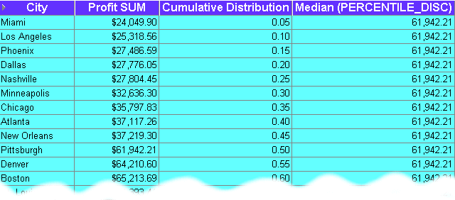
This example computes the median profit value for cities using the PERCENTILE_DISC function as a reporting aggregate function.
| Worksheet options | Set to: |
|---|---|
| Items | Video Analysis Information: City, Profit SUM |
| Sort Order | Not applicable |
| Conditions | Not applicable |
| Calculation Name | Median (PERCENTILE_DISC) |
| Calculation | PERCENTILE_DISC(0.5) WITHIN GROUP(ORDER BY Profit SUM) OVER() |
| Additional Calculations Required | Cumulative Distribution = CUME_DIST() OVER(ORDER BY Profit SUM) |
Figure A-27 Worksheet containing the Median(PERCENTILE_DISC) calculation

The worksheet shows the median profit value for cities. The median profit value (i.e. 0.50 in the Cumulative Distribution column) is $61,942,21 (i.e. the value for Pittsburgh, which has the value 0.50 in the Cumulative Distribution column).
Notes
On table worksheets, the calculation displays the returned value for each row in the worksheet. To return a single value, move the calculation into the Page Items area.
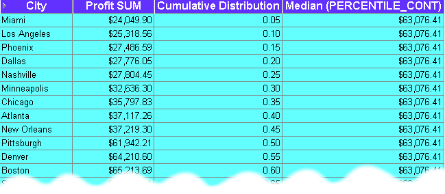
This example computes the median profit value for cities using the PERCENTILE_CONT function as a reporting aggregate function.
| Worksheet options | Set to: |
|---|---|
| Items | Video Analysis Information: City, Profit SUM |
| Sort Order | Not applicable |
| Conditions | Not applicable |
| Calculation Name | Median (PERCENTILE_CONT) |
| Calculation | PERCENTILE_CONT(0.5) WITHIN GROUP(ORDER BY Profit SUM) OVER() |
Figure A-28 Worksheet containing the Median(PERCENTILE_CONT) calculation

The worksheet shows the median profit value for cities. The median profit value is $63,076.41, which is the average profit value for the 0.50 and 0.55 percentile. In other words, the value for Pittsburgh plus the value for Denver, divided to two ($61,942.21 + $64,210.60)/2. For more information about how this function is calculated, see "About differences between PERCENTILE_CONT and PERCENTILE_DISC".
Notes
If the number of rows in the calculation is even, the two middle results are averaged. In the example above, the values for the .50 and .55 percentile are averaged.
On table worksheets, the calculation displays the returned value for each row in the worksheet. To return a single value, move the calculation into the Page Items area.
You use hypothetical rank and distribution functions for 'what-if?' analysis. These functions work out the position of a value if the value was inserted into a set of other values. For example, where would a person who generated sales of $1,200,000 be positioned in a ranked list of sales peoples' performance.
Note: You can also calculate the hypothetical values of the following:
DENSE_RANK - computes the rank of values where equal values receive the same rank (e.g. you can have more than one value ranked as top of the league)
CUME _DIST - computes the relative position of a specified value in a group of values
PERCENT_RANK - similar to CUME_DIST, this function calculates the rank of a value minus 1, divided by 1 less than the number of rows being evaluated
Examples:
This example calculates the hypothetical rank of profit values in relation to profit values for departments and regions. For example, to answer the question, how would a sales value of $500.00 be positioned in a ranked list of values for the Video Sale department in each region?
Note: This example uses a parameter to provide dynamic input to the calculation (for more information see "About using parameters to provide dynamic input to calculations").
| Worksheet options | Set to: |
|---|---|
| Items | Video Analysis Information: Calendar Year, Region, Department, Profit, Profit COUNT, Profit MAX, Profit MIN |
| Sort Order | Region (Lo to Hi) |
| Conditions | Not applicable |
| Page Items | Calendar Year=2000, Department=Video Sale, Value of Parameter Hypothetical Value=500 |
| Parameters | Hypothetical Value - this value is entered by the Discoverer user when the worksheet is opened or refreshed. |
| Calculation Name | League table |
| Calculation | RANK(:Hypothetical Value) WITHIN GROUP(ORDER BY Profit DESC NULLS FIRST) |
Figure A-29 Worksheet containing the League table calculation

The worksheet shows where the hypothetical value of $500 would rank in a ranked list of regions:
The hypothetical profit amount of $500 would rank number 2 in the Central region containing 520 profit values (range $13.49 to $537.78).
The hypothetical profit amount of $500 would rank number 7 in the East region containing 807 values (range $11.99 to $539.06).
Notice that because the hypothetical amount ($500) is greater than the Profit MAX amount in the West region ($484.01), the amount $500 has the hypothetical rank of number 1 for the West region.
Notes
The items Profit COUNT, Profit MAX, Profit MIN are not used in the calculation. They are displayed on the worksheet to help illustrate how the function is working. For example, if you can see that the Profit MAX value is $484.01 in the West region, you can see why a hypothetical value of $500.00 ranks as 1. This is because the hypothetical value is greater than the maximum value (i.e. the item Profit MAX).
The League table calculation uses the value of the :Hypothetical Value parameter, entered when the worksheet is opened or refreshed. In the example below, the Hypothetical Value (displayed in the Hypothetical amount page item) is set to 500. For more information about using parameter values in calculations, see "About using parameters to provide dynamic input to calculations".
The Rank function must take a non-aggregated value as an ORDER BY argument. For example, you could not perform this function on SUM(Profit) or Profit AVG.
As an alternative to setting the Hypothetical Value as a parameter, you could enter the rank value directly into the calculation as the Rank() argument. For example:
RANK(500) WITHIN GROUP(ORDER BY Profit DESC NULLS FIRST)
If you do not use a parameter, you will have to change the calculation to change the hypothetical value.
You use the Oracle9i WIDTH_BUCKET function to divide values into groups (sometimes called bands or buckets) according to their value (for more information, see "About banding"). For example, to group data for a bar graph.
Hint: You can also use the GREATEST and the CASE functions to calculate equi-width bands (see "Example: Banding by value (1)" and "Example: Banding by value (2)".
Examples:
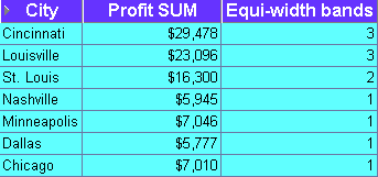
This example divides profit figures into three bands according to their value.
| Worksheet options | Set to: |
|---|---|
| Items | Video Analysis Information: City, Profit SUM |
| Sort Order | Equi-width bands |
| Conditions | Department = Video Sale OR Department = Video Rental
Calendar Year = 2000 Region = Central |
| Calculation Name | Equi-width bands |
| Calculation | WIDTH_BUCKET(Profit SUM,0,30000,3) |
Figure A-30 Worksheet containing the Equi-width bands calculation

The worksheet shows equi-width bands for profit values for cities. The first band (0 to 9,999) contains Nashville, Minneapolis, Dallas, and Chicago. The second band (10,000 to 19,999) contains St. Louis. The third band (20,000 to 30,000) contains Cincinnati and Louisville.
Notes
The WIDTH_BUCKET function takes four arguments:
worksheet item = Profit SUM
minimum value = 0
maximum value = 30000
number of bands = 3
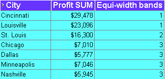
To assign bands in reverse order, reverse the minimum and maximum values. For example, WIDTH_BUCKET(Profit SUM,30000,0,3). This function produces the worksheet below.
Figure A-31 Worksheet containing the Equi-width bands calculation with reversed order

The worksheet shows equi-width bands for profit values for cities. The first band (20,000 to 30,000) contains Cincinnati and Louisville. The second band (10,000 to 19,999) contains St. Louis. The third band (0 to 9,999) contains Chicago, Dallas, Minneapolis, and Nashville.
You use FIRST/LAST aggregate functions to find the first or last value within an ordered group. This enables you to order data on one column but return another column. For example, to find the average sales transaction amount for the region with the largest number of sales transactions in a period.
Examples:
"Example: Find the largest sales transactions in area with most sales trans'"
"Example: Find the average sales transaction in area with least sales trans'"
Using FIRST/LAST functions maximizes Discoverer performance by avoiding the need to perform self-joins or sub-queries.
Note: You can use FIRST/LAST functions with the following:
MIN - find the smallest value in a list of values
MAX - find the largest value in a list of values
AVG - find the average value of a list of values
STDDEV - find the standard deviation of a list of values
VARIANCE - find the variance of a list of values
This example finds the largest sales transaction amount for the city with the most sales transactions in a period.
| Worksheet options | Set to: |
|---|---|
| Items | Video Analysis Information: City, Sales MAX, Sales Count |
| Sort Order | Not applicable
|
| Conditions | Department = Video Sale OR Department = Video Rental
Calendar Year = 2000 Region = Central |
| Calculation Name | Maximum sales in city with largest sales volume |
| Calculation | MAX(Sales MAX) KEEP(DENSE_RANK LAST ORDER BY Sales COUNT) OVER(PARTITION BY "Calendar Year", Region) |
Figure A-32 Worksheet containing the Maximum sales in city with largest sales volume calculation

The worksheet shows the largest sales transaction value in the city with the largest number of sales transactions. Cincinnati has the largest number of sales transactions (1220). The largest sales transaction for Cincinnati is $667.53.
Notes
Sales MAX - contains the largest sales transaction amount.
Sales COUNT - contains the number of sales transactions in the period.
To apply the function, Discoverer does the following:
orders the Sales COUNT column in the database (default order is ascending)
takes the last value in Sales COUNT column (i.e. the LAST argument), which is the largest number, and looks up the city name for this row (Cincinnati)
orders transactions in the database for Cincinnati and returns the LAST value, $667.53 (the default order is ascending)
The Sales COUNT and Sales MAX items are included to demonstrate that the calculation returns the correct result. The Sales COUNT and Sales MAX items are not used to calculate the result, which is calculated using aggregation in the database.
Hint: On table worksheets, the calculation displays the returned value for each row in the worksheet. To return a single value, move the calculation into the Page Items area.
This example calculates the average sales transaction amount for the city with the smallest number of sales transactions in a period.
| Worksheet options | Set to: |
|---|---|
| Items | Video Analysis Information: City, Sales COUNT, Sales AVG |
| Sort Order | Not applicable
|
| Conditions | Department = Video Sale OR Department = Video Rental
Region = Central Calendar Year = 2000 |
| Calculation Name | Average sales in city with smallest sales volume |
| Calculation | MIN(Sales AVG) KEEP(DENSE_RANK FIRST ORDER BY Sales COUNT) OVER(PARTITION BY "Calendar Year", Region) |
Figure A-33 Worksheet containing the Average sales in city with smallest sales volume calculation

The worksheet shows the average sales transaction value in the city with the smallest number of sales transactions. Nashville has the smallest number of transactions in the period (219). Therefore, the calculation returns the average transaction value for Nashville ($38.39).
Notes
Sales COUNT - contains the number of sales transaction in the period.
Sales AVG - contains the average sales transaction amount in the period.
To apply the function, Discoverer does the following:
orders the Sales COUNT column in the database (default order is ascending)
takes the first value in Sales COUNT column (i.e. the FIRST argument), which is the smallest number, and looks up the city name for this row (Nashville)
calculates the average sales value for Nashville, $38.39
The Sales COUNT and Sales AVG items are included to demonstrate that the calculation returns the correct result. The Sales COUNT and Sales AVG items are not used to calculate the result, which is calculated using aggregation in the database.
Hint: On table worksheets, the calculation displays the returned value for each row in the worksheet. To return a single value, move the calculation into the Page Items area.