| Bookshelf Home | Contents | Index | Search | PDF | |
Siebel Analytics Performance Tuning Guide > The Database Servers > Index Selection >
B-Tree Indexes
Generally speaking, in an online transaction processing environment, a B-tree is most effective when it is highly selective. When this is the case, the index is said to have "high selectivity" because a low percentage of rows in the table have the same index key value.
General Guidelines
With high selectivity in mind, evaluate creating B-tree indexes on columns that:
- Occur frequently in WHERE clauses
- Often used to join tables (include aggregate tables)
- Occur in ORDER BY clauses (the index can facilitate ordering)
- Occur in a foreign key reference constraint
- Used to enforce PRIMARY KEY and UNIQUENESS constraints
You can also look at your query workload and identify families of queries that include tight table constraints on tables (point, multi-point, and range queries).
When you have star schemas, both DB2 and Oracle database servers can exploit multi-column B-Tree indexes to accelerate join processing when they are created over the foreign key reference columns of "fact" tables. DB2 and Oracle can also accelerate star join operations when single column indexes are created on the fact table's foreign key reference columns. In the Oracle case, these indexes are specialized Bitmap indexes which are used by the server's star transformation algorithm. See Bitmap Indexes.
Where B-Trees Should Not Be Created
Several situations are worth noting where you should not create B-Tree indexes on columns. These cases include columns which:
- Have only a few distinct values in their domains. For example, a Type column that has only four distinct values (A, B, C, and D). The index would be said to have "low selectivity." If you have an Oracle database, then these columns of low selectivity are ideal candidates for Bitmap indexes.
- Occur in WHERE clauses but within functions other than MIN or MAX.
Indexes in these cases waste space and slow down the load process.
Siebel Recommended Methodology
You can follow the methodology described in the following example procedure to create new indexes to speed up a slow running report. The slow running report used in this example is "Abandoned Carts Detail."
To analyze a slow running report
- Log into Siebel Analytics and run the Abandoned Carts Detail report.
- Click the Results tab.
- After waiting for unacceptably long period of time, cancel the query.
- Trace the SQL using the Siebel Analytics Admin Mode.
- Return to the dashboard.
- Click the Admin hyperlink.
Analytics returns the Siebel Analytics Administration page.
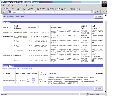
- Click the Manage Sessions hyperlink.
Analytics returns the Sessions page shown in the figure below.
- Look in the Cursor Cache window for your session.
In this case, there is only one session in the window and it ran 2 minutes and 52 seconds.
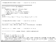
- Click the View Log hyperlink.
Analytics returns another window that contains the SQL generated for the session, the logical SQL inside the Analytics server and the SQL sent to the database, which is shown in the following sections.
Note the time between each section marked by lines such as:
+++Administrator:30000:30002:----2002/07/01 22:20:42In the screen shot below, note that the mean time between these lines is just short of 3 minutes.
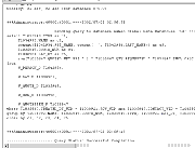
- Run the SQL sent to the database using the EXPLAIN PLAN command.
You can generate the execution plan for a query in a variety of ways such as SQL*Plus, Oracle Enterprise Manager, or TOAD (Tools for Oracle Application Development). This example copies and pastes the SQL into TOAD.
The figure below shows the generated SQL in a TOAD window.
The SQL text including the explain plan output was copied and pasted on the next page.
select T1035949.TYPE as c1,
T1034992.NAME as c2,
concat(T1042934.FST_NAME,
concat(' ', T1042934.LAST_NAME)) as c3,
T1035949.QUOTE_NUM as c4
T1038921.DAY_DT as c5,
sum(T1035847.QUOTED_NET_PRI * 1 * T1035847.QTY_REQUESTED
* T1035847.INCL_CALC_IND - T1035847.ADJUSTMENT
+ T1035847.FREIGHT_AMT + T1035847.TAX_AMT) as c6
from W_PERSON_D T1042934, W_DAY_D T1038921, W_QUOTE_D T1035949, W_ORG_D
T1034992, W_QUOTEITEM_F T1035847
where T1035847.CREATED_DT_WID = T1038921.ROW_WID
and T1035847.CONTACT_WID = T1042934.ROW_WID
and T1035847.QUOTE_WID = T1035949.ROW_WID
and T1034992.ROW_WID = T1035847.TGT_ACCNT_WID
and T1034992.ACCNT_FLG = 'Y'
group by T1034992.NAME, T1035949.QUOTE_NUM, T1035949.TYPE,
T1038921.DAY_DT, T1038921.INTEGRATION_ID, T1042934.INTEGRATION_ID,
concat(T1042934.FST_NAME, concat(' ',T1042934.LAST_NAME))
order by c1, c2, c3, c4, c5SELECT STATEMENT Optimizer=ALL_ROWS (Cost=2325184460 Card=1880231459032250
Bytes=691925176923868000)
SORT (GROUP BY) (Cost=2325184460 Card=1880231459032250
Bytes=691925176923868000)
HASH JOIN (Cost=88222326 Card=1880231459032250 Bytes=691925176923868000)
TABLE ACCESS (FULL) OF W_PERSON_D (Cost=22838 Card=3520816
Bytes=295748544)
HASH JOIN (Cost=392 Card=8010492990 Bytes=2274980009160)
TABLE ACCESS (FULL) OF W_DAY_D (Cost=10 Card=6325 Bytes=246675)
HASH JOIN (Cost=39 Card=18997217 Bytes=4654318165)
TABLE ACCESS (FULL) OF W_QUOTE_D (Cost=25 Card=17394 Bytes=817518)
NESTED LOOPS (Cost=5 Card=16383 Bytes=3243834)
TABLE ACCESS (FULL) OF W_QUOTEITEM_F (Cost=1 Card=15 Bytes=1950)
TABLE ACCESS (BY INDEX ROWID) OF W_ORG_D (Cost=1 Card=16383
Bytes=1114044)
INDEX (UNIQUE SCAN) OF W_ORG_D_P1 (UNIQUE)The processing costs for each operation within the query is a relative estimate which highlights the costliest operations within the query. These are the operations that you need to analyze closely.
The most expensive table to access within this plan is to W_PERSON_D. This also happens to be the largest table in the test database (4 GB). If the hash area of the columns from this table can be reduced, this will reduce access time.
One method to reduce this access time is to index the columns in the table so that the query scans the indexes instead of the table.
- Locate all occurrences of the table's columns within the query.
The columns FST_NAME and LAST_NAME occur in the query's select list and the column ROW_WID occurs in its where clause.
- Create and analyze an index that covers these columns.
Create index w_person_d_x7
on w_person_d (row_wid, fst_name, last_name)
tablespace idx nologging pctfree 0 ;Analyze index w_person_d_x7 compute statistics ;
TIP: The columns referenced in the WHERE clause should be the leading columns for a particular index. If the columns were created in another order, say (LAST_NAME, FST_NAME, ROW_WID), the optimizer would not generate a query that uses the index.
- Generate the explain plan for the query and compare query plans.
SELECT STATEMENT Optimizer=ALL_ROWS (Cost=2325173878 Card=1880231459032250
Bytes=691925176923868000)
SORT* (ORDER BY) (Cost=2325173878 Card=1880231459032250
Bytes=691925176923868000)
SORT* (GROUP BY) (Cost=2325173878 Card=1880231459032250
Bytes=691925176923868000)
SORT* (GROUP BY) (Cost=2325173878 Card=1880231459032250
Bytes=691925176923868000)
HASH JOIN* (Cost=88211744 Card=1880231459032250
Bytes=691925176923868000)
VIEW* OF index$_join$_001 (Cost=12256 Card=3520816 Bytes=295748544)
HASH JOIN* (Cost=88211744 Card=1880231459032250
Bytes=691925176923868000)
INDEX* (FAST FULL SCAN) OF W_PERSON_D_X7 (NON-UNIQUE)
(Cost=1 Card=3520816 Bytes=295748544)
INDEX* (FAST FULL SCAN) OF W_PERSON_D_U1 (UNIQUE)
(Cost=1 Card=3520816 Bytes=295748544)
HASH JOIN* (Cost=392 Card=8010492990 Bytes=2274980009160)
TABLE ACCESS (FULL) OF W_DAY_D (Cost=10 Card=6325 Bytes=246675)
HASH JOIN (Cost=39 Card=18997217 Bytes=4654318165)
TABLE ACCESS (FULL) OF W_QUOTE_D (Cost=25 Card=17394
Bytes=817518)
NESTED LOOPS (Cost=5 Card=16383 Bytes=3243834)
TABLE ACCESS (FULL) OF W_QUOTEITEM_F (Cost=1 Card=15
Bytes=1950)
TABLE ACCESS (BY INDEX ROWID) OF W_ORG_D (Cost=1 Card=16383
Bytes=1114044)
INDEX (UNIQUE SCAN) OF W_ORG_D_P1 (UNIQUE)The plan shows that the full table scan of the W_PERSON_D was replaced with a hash join of two indexed lookups.
- Verify the performance improvement.
Copy the query from the explain plan, paste it into TOAD, and then execute the query with TOAD. The elapsed time reported by TOAD is now 48 seconds. This is roughly one-fourth the original time.
- Flush the query cache from the Analytics server.
Navigate to the Admin View - Manage Session, and click the Close All Cursors hyperlink.
- Run the Analytics report again.
- Return to Admin mode and verify that the report ran faster (47 seconds).
Thus, a multicolumn B-Tree index on the W_PERSON_D dimension table improves query performance roughly 300 percent.
| Bookshelf Home | Contents | Index | Search | PDF | |
Siebel Analytics Performance Tuning Guide Published: 18 April 2003 |