| Oracle® Retail Demand Forecasting Implementation Guide Release 16.0 |
|

 Previous |
 Next |
This appendix details these topics:
The purpose of the Oracle Retail Preprocess module, which may also be referred to as Preprocessing, is to correct past data points that represent unusual sales values that are not representative of a general demand pattern. Such corrections may be necessary when an item is out of stock and cannot be sold, which usually results in low sales. Preprocessing will adjust for stock out for both the current week and the following week because it assumes that the out of stock indicators represent end of week stock out. Data Correction may also be necessary in a period when demand is unusually high. The Preprocess module allows you to automatically make adjustments to the raw POS (Point of Sales) data so that subsequent demand forecasts do not replicate undesired patterns that are caused by lost sales or unusually high demand.
The Preprocess Syntax section contains the specifications and syntax for configuring the Preprocess function in the RPAS Configuration Tools. There is an RPAS multi-return function named preprocess and one RPAS special expression named preprocess. The special expression provides better performance; however, it only works in the batch mode. The multiple return function preprocess works in both batch mode and workbook mode. The syntax is exactly the same in both modes, except that procedures use <- instead of = in the expression.
|
Note: The syntax is slightly different than the standard RPAS functions and procedures that are described in the Rule Functions Reference Guide section of the Oracle Retail Predictive Application Server Configuration Tools User Guide. |
The following libraries must be registered in any domains that will use the Preprocess solution extension:
AppFunctions
PreprocesssFunctions
The following restrictions apply to use the Preprocess function/procedure:
An underscore (_) character may not be used in any measure names and rules unless the measures and rules are to be expanded using the RDF or Curve solution's classification scheme.
The classifications apply the AppFunctions and are as follows:
_F: Expand measures and rules across final levels
_S: Expand measures and rules across source levels
_B: Expand measures and rules across birth dates
The following models require that the stated measure is to be provided.
Bayesian model—Plan measure required.
Profile model—Profile measure required.
The following notes are intended to serve as a guide for configuring the Preprocess function within the RPAS Configuration Tools:
The Preprocess function is an RPAS C++ special expression. In order to get multiple results, the resultant measures must be configured in the Measure Tool, and the specific measure label must be used on the left-hand side (LHS) of the function call. The resultant measure parameters must be comma-separated in the function call as in the example.
Because different filtering methods require different input parameters, it is necessary that every input parameter (measure or constant) must be accompanied by the corresponding label. All of the input measure parameters must be configured and registered before the function call. The input parameters must be comma-separated in the function call as in the example.
The Preprocess function library must be registered after the domain build by using the regfunction RPAS utility.
The Preprocess function required all the input and output measures using the same intersections. Mixed input/output measure intersections should be aligned to the same calculation intersection with other RPAS function/procedure before calling the Preprocess function. The same procedure can be carried out to the resultant measures to spread or aggregate them to the designated intersections.
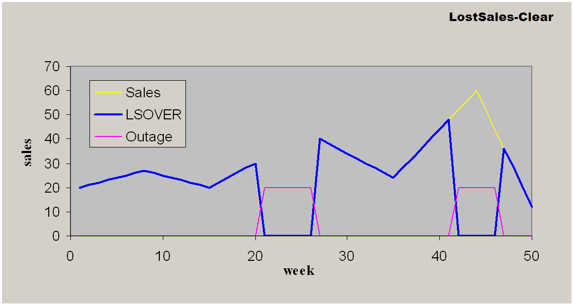
Because of the limitation that the same measure cannot simultaneously appear on both left-hand side and right-hand side, the implementation of the CLEAR filter requires the user to provide a LSOVER_REF measure (a duplication of the previously calculated LSOVER measure) when you try to retain the results on certain time series but clear the others by providing a mask measure (TSMASK_DENSE). The LSOVER_REF is not required when the results for all the time series need to be cleared.
The LSTODAY measure is used to specify the end date for the filter processing. It only accepts the index number for the end date along the calendar dimension as valid input. If it is desired that the string position name to be used for the end date specification, the available RPAS time dimension translation function index can be used to do the name-index conversion before calling the Preprocess function.
The LSTODAY input parameter is designed to be a measure rather than a constant to provide more flexibility. Current implementation only allows one global LSTODAY index value to be used in processing all the time series. To specify the end date, you just need to populate its value for the first time series, and this index will be applied to all the other time series.
The index value in the LSTODAY measure starts from 0.
FLP_FIRST and FLP_LAST are the resultant measures to be used for the First-Last-Populated Location calculation. They do not have the calendar dimension, and each of their cell values represent the indices for the first and last populated locations along the calendar dimension from the first time series up to the current time series, respectively.
TSMASK_DENSE is a Boolean input measure without calendar dimension to specify which time series is going to be processed and which is not. For filtering methods other than the CLEAR method, the true value means that it will be processed if the popcount for the current time series is larger than the hard-coded threshold value. Otherwise, it will not be processed. The false value means that the current time series will not be processed. If the TSMASK_DENSE measure is not specified, all the time series will be processed and the internal hard-coded threshold value will not be considered. For the CLEAR filtering method, the true value means that the previously calculated results for the current time series will be cleared and the false value means the results will be retained. If the TSMASK_DENSE measure is not specified, all the results will be cleared.
For all the input measures that do not have the calendar dimension, such as UP_ADJ_RATIO and DELTA, you can use a constant as input. In this case, the constant value will be applied to all the time series.
The syntax for using the Preprocess is shown in the following examples. The input and output parameter tables explain the specific usage of the parameters names use in the function/procedure.
Example E-1 Generic Example 1:
LSOVER: LSOVERMEAS, LS: LSMEAS, [, TSALERT: TSALERTMEAS, SERVICE_LEVEL: SERVICELEVELMEAS, STOCK_LEVEL: STOCKLEVELMEAS, FLP_FIRST: FLPFIRSTMEAS, FLP_LAST: FLPLASTMEAS] <- preprocess(SRC: SRCMEAS, LSTODAY: LSTODAYMEAS, NPTS: NPTSMEAS [, MIN_TSALERT: MINTSALERTMEAS, OUTAGE: OUTAGEMEAS, TSMASK_DENSE: TSMASKMEAS, UP_ADJ_RATIO: UPADJMEAS, DOWN_ADJ_RATIO: DOWNADJMEAS, REFERENCE: REFMEAS, DEVIATION: DEVMEAS {, WINDOW: WINDOWMEAS |, WINDOW1: WINDOW1MEAS, WINDOW2: WINDOW2MEAS, WINDOW3: WINDOW3MEAS, WINDOW4: WINDOW4MEAS, WINDOW5: WINDOW5MEAS} {, ALPHA: ALPHAMEAS, NPAST: NPASMEAS, NFUT: NFUTMEAS} {, NSIGMA_MIN: NSIGMA_MINMEAS, NSIGMA_MAX: NSIGMA_MAXMEAS |, NSIGMAOUT_MIN: NSIGMAOUT_MINMEAS, NSIGMAOUT_MAX: NSIGMAOUT_MAXMEAS, NSIGMAADJ_MIN: NSIGMAADJ_MINMEAS, NSIGMAADJ_MAX: NSIGMAADJ_MAXMEAS} {, FRCST_MIN: FRCST_MINMEAS, HIST_MIN_FS: HIST_MIN_FSMEAS} {, PRICE: PRICEMEAS, INVENTORY: INVENTORYMEAS, HIST_MIN_MD: HISTMINMDMEAS}, DELTA: DELTAMEAS, LSOVER_REF: LSOVERREFMEAS]
Example E-2 Generic Example 2:
LSOVER: LSOVERMEAS, LS: LSMEAS, [, TSALERT: TSALERTMEAS, SERVICE_LEVEL: SERVICELEVELMEAS, STOCK_LEVEL: STOCKLEVELMEAS, FLP_FIRST: FLPFIRSTMEAS, FLP_LAST: FLPLASTMEAS] <-preprocess(SRC: SRCMEAS, LSTODAY: LSTODAYMEAS, NPTS: NPTSMEAS [, MIN_TSALERT: MINTSALERTMEAS, OUTAGE: OUTAGEMEAS, TSMASK_DENSE: TSMASKMEAS, UP_ADJ_RATIO: UPADJMEAS, DOWN_ADJ_RATIO: DOWNADJMEAS, REFERENCE: REFMEAS, DEVIATION: DEVMEAS {, WINDOW: WINDOWMEAS |, WINDOW1: WINDOW1MEAS, WINDOW2: WINDOW2MEAS, WINDOW3: WINDOW3MEAS, WINDOW4: WINDOW4MEAS, WINDOW5: WINDOW5MEAS} {, ALPHA: ALPHAMEAS, NPAST: NPASMEAS, NFUT: NFUTMEAS} {, NSIGMA_MIN: NSIGMA_MINMEAS, NSIGMA_MAX: NSIGMA_MAXMEAS |, NSIGMAOUT_MIN: NSIGMAOUT_MINMEAS, NSIGMAOUT_MAX: NSIGMAOUT_MAXMEAS, NSIGMAADJ_MIN: NSIGMAADJ_MINMEAS, NSIGMAADJ_MAX: NSIGMAADJ_MAXMEAS} {, FRCST_MIN: FRCST_MINMEAS, HIST_MIN_FS: HIST_MIN_FSMEAS} {, PRICE: PRICEMEAS, INVENTORY: INVENTORYMEAS, HIST_MIN_MD: HISTMINMDMEAS}, DELTA: DELTAMEAS]
Table E-1 provides the input parameters for the Preprocess procedure.
Table E-1 Input Parameters for the Preprocess Procedure
| Parameter Name | Description |
|---|---|
|
SRC |
The source data. Data Type: Real Required: Yes |
|
METHODID |
The filtering method ID. Data Type: Real Required: Yes |
|
LSTODAY |
The end date for filter processing. Data Type: Real Required: Yes |
|
NPTS |
The number of points into history that will be filtered. Data Type: Real Intersection: Required: Yes |
|
MIN_TSALERT |
The threshold value used to set off TSALERT. Data Type: Real Required: No |
|
OUTAGE |
The outage indicator. Data Type: Boolean Required: No |
|
TSMASK_DENSE |
A Boolean value to specify which time series will be processed. Data Type: Boolean Required: No |
|
UP_ADJ_RATIO |
The upward adjustment ratio that will be applied on LS. Data Type: Real Required: No Default value: 1.0* * If the measure is not specified, the default value will be applied to each of the time series to be processed. |
|
DOWN_ADJ_RATIO |
The downward adjustment ratio that will be applied on LS. Data Type: Real Required: No Default value: 1.0* * If the measure is not specified, the default value will be applied to each of the time series to be processed. |
|
REFERENCE |
Reference will be used for source data substitution. Data Type: Real Required: No |
|
DEVIATION |
The standard deviation for confidence interval calculation by Forecast Sigma filters. Data Type: Real Required: No |
|
WINDOW |
Filter window length for Standard Median filter. Data Type: Real Required: No Default value: 13 |
|
WINDOW1 |
First round filter window length for Oracle Retail Median filter. Data Type: Real Required: No Default value: 13 |
|
WINDOW2 |
Second round filter window length for Oracle Retail Median filter. Data Type: Real Required: No Default value: 19 |
|
WINDOW3 |
Third round filter window length for Oracle Retail Median filter. Data Type: Real Required: No Default value: 7 |
|
WINDOW4 |
Forth round filter window length for Oracle Retail Median filter. Data Type: Real Required: No Default value: 5 |
|
WINDOW5 |
Fifth round filter window length for Oracle Retail Median filter. Data Type: Real Required: No Default value: 11 |
|
ALPHA |
The exponential coefficient used to evaluate past and future velocities. Data Type: Real Required: No Default value: 0.2 |
|
NPAST |
The maximum number of historical points to calculate past velocity. Data Type: Real Required: No Default value: 5 |
|
NFUT |
The maximum number of historical points to calculate future velocity. Data Type: Real Required: No Default value: 5 |
|
NSIGMA_MIN |
The number of standard deviations for lower bound calculation. Data Type: Real Required: No Default value: 3.0 |
|
NSIGMA_MAX |
The number of standard deviations for upper bound calculation. Data Type: Real Required: No Default value: 3.0 |
|
FRCST_MIN |
The forecast lower bound for Forecast Sigma filters. Data Type: Real Required: No Default value: 0.1 |
|
HIST_MIN_FS |
The minimum number of historical points required for Forecast Sigma filters. Data Type: Real Required: No Default value: 5 |
|
NSIGMAOUT_MIN |
The number of standard deviations for lower outlier calculation. Data Type: Real Required: No Default value: 3.0 |
|
NSIGMAOUT_MAX |
The number of standard deviations for upper outlier calculation. Data Type: Real Required: No Default value: 3.0 |
|
NSIGMAADJ_MIN |
The number of standard deviations for lower bound calculation. Data Type: Real Required: No Default value: 1.5 |
|
NSIGMAADJ_MAX |
The number of standard deviations for upper bound calculation. Data Type: Real Required: No Default value: 1.5 |
|
DELTA |
Ratio of reference will be used to copy or increase for OVERRIDE and INCREMENT filters. Data Type: Real Required: No Default value: 1.0* * If the measure is not specified, the default value will be applied to each of the time series to be processed. |
|
LSOVER_REF |
Data will be used to override SRC. Used by CLEAR filter only. Data Type: Real Required: No |
|
POA |
Partial Outage Flag. Used by STD ES LS filter only. If set to False, the period immediately following an out-of-stock period will not be adjusted. The default value is True. Data Type: Boolean Required: No |
|
EVENT_FLAG |
Used by STD ES and STD ES LS filters. If a value is True, the given period is not used in the calculation of the past or future velocities. Data Type: Boolean Required: No |
|
STOP_AT_EVENT FLAG |
Used by STD ES and STD ES LS filters. This parameter determines which periods are included in the calculation of past/future velocities. If the flag is set to True, then the algorithm only includes periods before the first event flag or event indicator. If the flag is set to False, then all available, non-flagged periods, within the windows defined by nfut and npast, are used in the calculation of the past and future velocities. The default setting for the flag is False |
|
SRCPOPCUT |
The minimum number of non-zero sales data points in the preprocessing window. If the non-zero sales data points number is less than this parameter, then the time series is not processed. Data Type: Numeric Required: No. If this parameter is not provided, it defaults to 3 in the code. |
Table E-2 provides the output parameters for the Preprocess function/procedure.
Table E-2 Output Parameters for the Preprocess Procedure
| Parameter Name | Description |
|---|---|
|
LSOVER |
Adjusted source data. It is the Primary Result. LSOVER = SRC + LS Data Type: Real Required: Yes |
|
LS |
The adjustment on the source data. Data Type: Real Required: Yes |
|
TSALERT |
Boolean flag set to True when more than MIN_TSALERT number of data points have been modified. Data Type: Boolean Required: No |
|
SERVICE_LEVEL |
SERVICE_LEVEL = SRC / LSOVER Data Type: Real Required: No |
|
STOCK_LEVEL |
Used by Mark Down filter only. Data Type: Real Required: No |
|
FLP_FIRST |
First populated position. Used by FLP filter only. Data Type: Real Required: No |
|
FLP_LAST |
Last populated position. Used by FLP filter only. Data Type: Real Required: No |
Table E-3 provides the numeric value assigned to the forecast model/model list.
Table E-3 Numeric Values Assigned to the Lost Sales Model/Model List
| Model | Numeric Value | Comments |
|---|---|---|
|
MEDIAN5 |
0 |
Oracle Retail Median. Required input parameters: None Optional input parameters:
|
|
MEDIAN1 |
1 |
Standard Median. Required input parameters: None Optional input parameters: WINDOW |
|
OVERRIDE |
2 |
Override Required input parameters: REFERENCE Optional input parameters: DELTA |
|
INCREMENT |
3 |
Increment. Required input parameters: REFERENCE Optional input parameters: DELTA |
|
ES_LT |
4 |
Standard ES. Required input parameters: OUTAGE Optional input parameters:
|
|
LS_ES_LT |
9 |
Lost Sales—Standard ES. Required input parameters: OUTAGE Optional input parameters:
|
|
FRCST_SIGMA |
14 |
Forecast and standard deviation algorithm. Required input parameters:
Optional input parameters:
|
|
FRCST_SIGMA_EVENT |
15 |
Forecast and standard deviation algorithm with Event. Required input parameters:
Optional input parameters: NSIGMAOUT_MAX
|
|
CLEAR |
17 |
Clear—clears specified result measures. Required input parameters: None Optional input parameters:
|
|
NO_FILT |
19 |
No filtering. Required input parameters: None Optional input parameters: None |
|
DEPRICE |
22 |
Remove pricing effects Required input parameters:price, maximum price Optional input parameters:none |
|
FLP: first populated location |
20 |
Required input: src and method |
This section details the following Preprocess filtering methods:
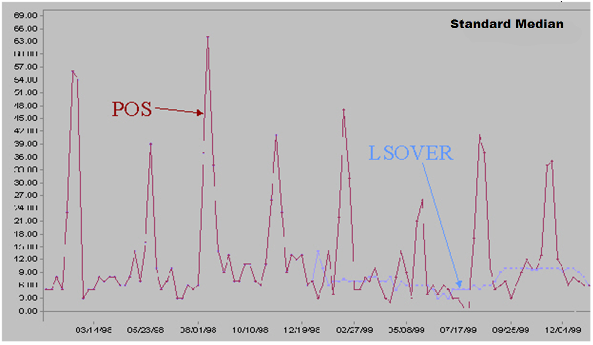
Standard Median is recommended for getting data baselines on long time ranges when promo indicators are not available.
A standard median filter implementation:
Does not take outage information as an input.
Can use one optional parameter: window length.
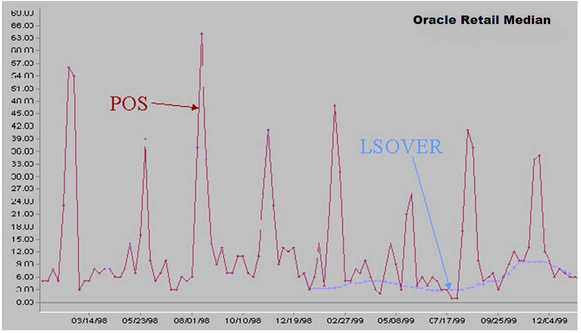
Oracle Retail Median is recommended for getting data baselines on long time ranges when promo indicators are not available.
Oracle Retail Median provides the following features:
A sophisticated median filter that takes trends into consideration and improves side effects over the standard median filter. It makes five standard median filter passes.
Does not take outage information as an input.
Can accept five optional parameters: window length for each pass.
The first two passes recursively apply the standard median filter. The result is denoted by MEDIAN_2(t). The one-step difference of MEDIAN_2(t) is calculated. That is, DIFF_1(t) = MEDIAN_2(t) - MEDIAN_2(t-1). Then, the standard median filter is applied to DIFF_1(t). The result is denoted by MEDIAN_DIFF_1(t).
Using MEDIAN_DIFF_1(t), a first smoothed version (that is, baseline) of the source data is calculated at the third step: SMOOTH_1(t) = SMOOTH_1(t-1) + MEDIAN_DIFF_1(t) on points where the absolute deviation of SRC(t) over its mean is larger than half of the global absolute standard deviation. Otherwise, SMOOTH_1(t) = SRC(t).
To prepare for the fourth pass, the one-step difference of SMOOTH_1(t) is calculated. That is, DIFF_2(t) = SMOOTH_1(t) - SMOOTH_1(t-1). An average version of DIFF_2(t) is calculated using the standard median filter. The result is denoted by AVG_DIFF_2(t). The result of the fourth pass is SMOOTH_2(t) = SMOOTH_2(t-1) + AVG_DIFF_2(t).
Finally, LSOVER(t) is the result of applying the standard median filter to SMOOTH_2(t).
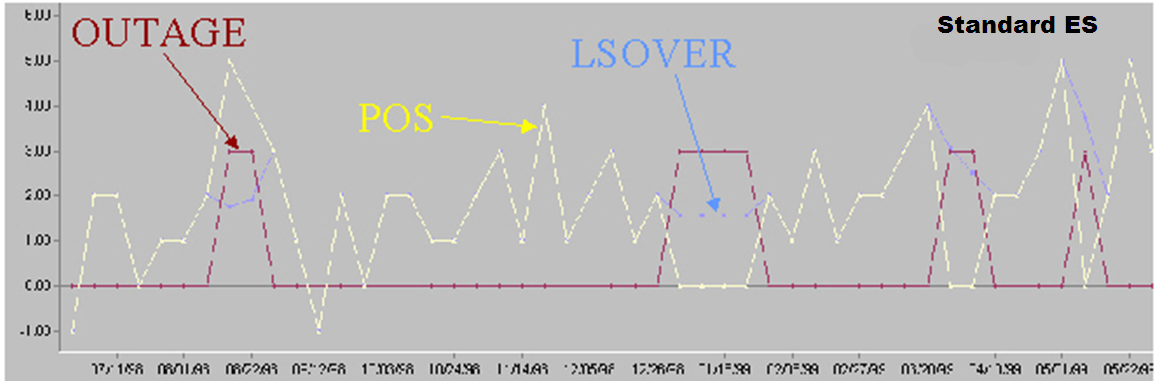
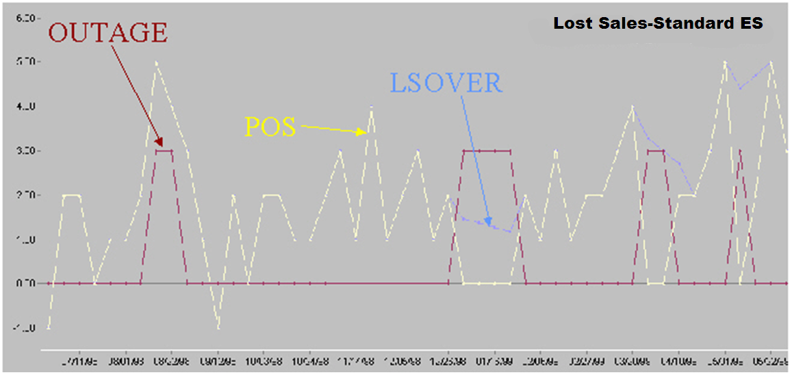
Standard Exponential Smoothing (Std ES) removes spikes (such as promotional promo, temporary price changes, and so on), as well as filling the gaps (out of stock, unusual events such as a fire or hurricane).
Input: An Event Indicator that indicates which periods should be preprocessed.
Optional Parameters:
The following table details the optional parameters for Standard Exponential Smoothing.
| Optional Parameters | Description |
|---|---|
| ES (Exponential Smoothing) | The alpha parameter that determines the weight put on observations of periods included in the calculations. |
| Number of future periods (nfut) | The number of periods after an outage periods that are considered in the calculation of the future velocity.
Note that if during these periods an event flag or a event indicator is on, the particular period is excluded from the calculation. |
| Number of past periods (npast) | The number of periods before an outage periods that are considered in the calculation of the past velocity.
Note: When calculating the past velocity and the first period in the preprocessing window is flagged, then the past velocity is calculated using earlier periods outside the preprocessing window. Note that if during these periods an event flag or a event indicator is on, the particular period is excluded from the calculation. |
| Event flag | This parameter indicates if a period should be excluded from the calculation of past/future velocities. |
| Stop at event flag | This parameter determines which periods are included in the calculation of past/future velocities.
If the flag is set to True, then the algorithm only includes periods before the first event flag or event indicator. If the flag is False, then all available, non-flagged periods, within the windows defined by nfut and npast, are used in the calculation of the past and future velocities. The default setting for the flag is False. |
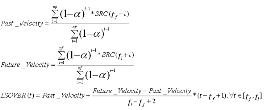
Std ES is the standard Exponential Smoothing filter. It preprocesses a subset of points as predetermined by an input measure. For every contiguous sequence of points to adjust, say between tf and tl, a past velocity and a future velocity are calculated using an exponentially weighted average. For the points between tf and tl, the adjustment is calculated as a linear interpolation of the past and future velocities.
Where:
 |
is the exponential coefficient used to evaluate past and future velocities. |
|
 |
is the maximum number of historical points to calculate past velocity. |
|
 |
is the maximum number of future points to calculate future velocity. |
Lost Sales—Standard Exponential Smoothing functions like Std ES with two exceptions. First, it only adjusts lost sales (that is, negative spikes). Second, it can adjust not only the out-of-stock period but also the period immediately following such a period (partial outage period).
Forecast Sigma is recommended for removing recent spiky data points when approved forecasts and approved confidence intervals are available on the filtering window, but spike indicators are not available. This method is based on the principle that if a data point significantly deviates from an approved forecast, this data point is likely to be an unusual event that should be overridden in the source measure (POSOVER) used by the forecasting engine. It is adjusted by bringing the override value within some bounds of the approved forecast as defined by a proportional coefficient scalar of the forecasts' standard deviation.
Forecast Sigma provides the following features:
Does not take outage information as an input
Requires two parameters:
Approved forecast array
Approved standard deviation array of forecast
Can accept four optional parameters:
Number of standard deviations for upper bound
Number of standard deviations for lower bound.
Forecast lower bound
Minimum item history (# points) required for filtering
This method relies on approved forecasts with their corresponding confidence intervals. It adjusts the points that are far (as defined by a multiple of the forecast standard deviation) from their corresponding previously approved forecasts by bringing the override values to their closest confidence interval bounds.
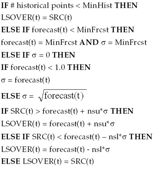
Where:
nsu is the number of standard deviations for upper bound.
nsl is the number of standard deviations for lower bound.
MinFrcst is the forecast lower bound.
MinHist is the minimum item history (# points) required for filtering.
Example E-9 Lost Sales—Forecast Sigma with nsu = 3, nsl = 3, minFrcst = 0.1 and minHist = 5 weeks
LSOVER:LSOVER1, LS:LS1, TSALERT:TSALERT1 <- preprocess(SRC:POS, METHODID:mthid, LSTODAY:TODAY1, NPTS:npts, REFERENCE:forecast1, DEVIATION:dev1, NSIGMA_MIN:nsigma_min, NSIGMA_MAX:nsigma_max, FRCST_MIN:0.1, HIST_MIN_FS:hist_min_fs)
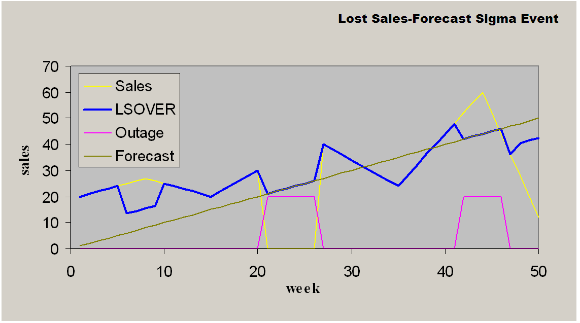
This is similar to Forecast Sigma. It takes an outage (for instance, event) indicator to further process.
When the outage/event mask is ON:
LSOVER(t) = forecast(t)
When the outage/event mask is OFF:
If the data points that are outside of the outliers calculated through NSIGMAOUT_MIN and NSIGMAOUT_MAX, they will be brought into the confidence interval bounds, which are defined through NSIGMAADJ_MIN and NSIGMAADJ_MAX.
Lost Sales—Forecast Sigma Event with nsigmaout_min = 3, nsigmaout_max = 3, nsigmaadj_min = 1.5, nsigmaadj_max = 1.5, minFrcst = 0.1 and minHist = 5 weeks
Example E-10 Lost Sales—Forecast Sigma Event
LSOVER:LSOVER1, LS:LS1, TSALERT:TSALERT1 <- preprocess(SRC:POS, METHODID:mthid, LSTODAY:TODAY1, NPTS:npts, OUTAGE:outage1, REFERENCE:forecast1, DEVIATION:dev1, NSIGMAOUT_MIN:nsigmaout_min, NSIGMAOUT_MAX:nsigmaout_max, NSIGMAADJ_MIN:nsigmaadj_min, NSIGMAADJ_MAX:nsigmaadj_max, FRCST_MIN:frcst_min, HIST_MIN_FS:hist_min_fs)
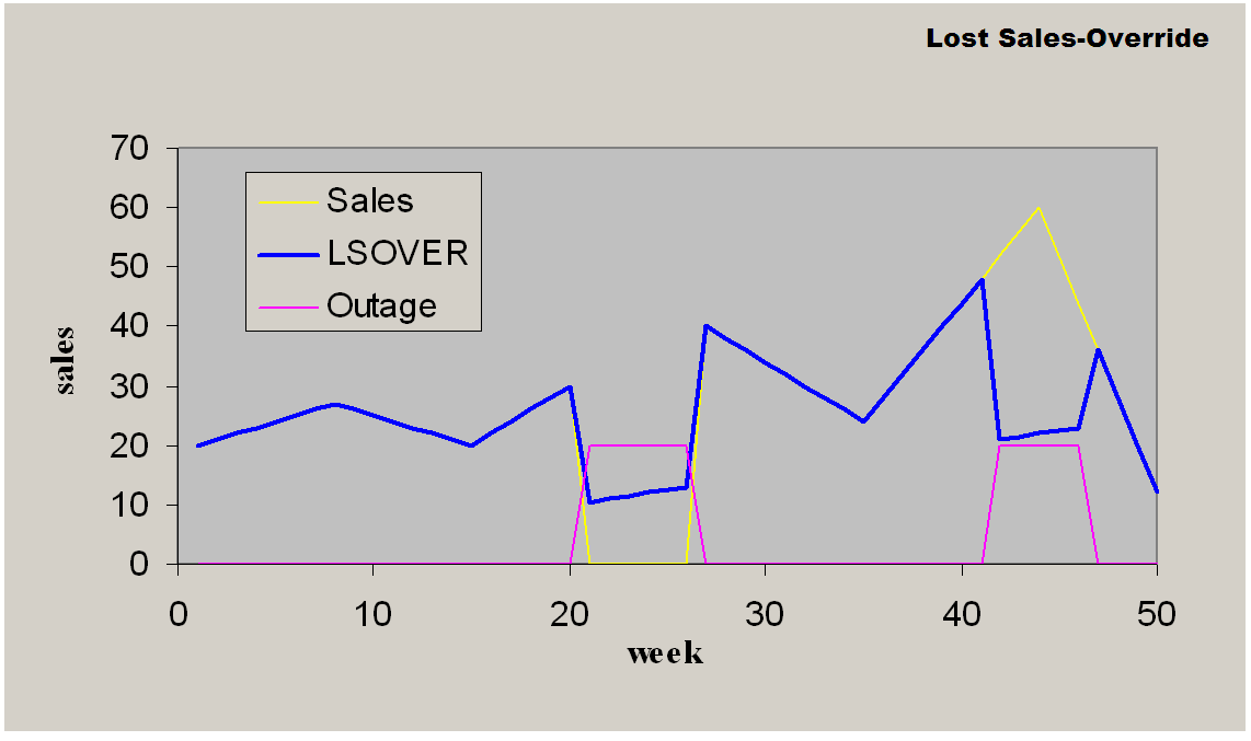
This method overrides the destination measure with the source measure that is adjusted by the adjustment percentage according to the mask. It is recommended for filling data gaps when an existing reference measure exists as a default value.
Override provides the following features:
It is a simple data copy of a given percentage of the reference data to copy from.
This may or may not take outage (for instance, event) info as an input to mask the operation.
Requires two parameters:
Reference measure to copy data from
Source measure for the original data
Can accept one optional parameter, Ratio of reference to actually copy.
This method uses the following parameters:
A source measure that can be any measure in the system as long as it has the same intersection as the destination measure
A reference measure that can be any measure in the system as long as it has the same intersection as the destination measure
A destination measure that can be any measure in the system as long as it has the same intersection as the source measure
A mask that is a Boolean measure that has the same intersection as the source and destination measures
An adjustment percentage
This method overrides the destination measure with the source measure adjusted by the adjustment percentage according to the mask:
Let:
S(i) is the value in cell (i) of the source measure
R(i) is the value in cell (i) of the reference measure
D(i) is the value in cell (i) of the destination measure
M(i) is the value of cell (i) of the mask
a is an adjustment percentage
The result of the override method is:
D(i) = a * R(i) if M(i) is True
D(i) = S(i) if M(i) is False
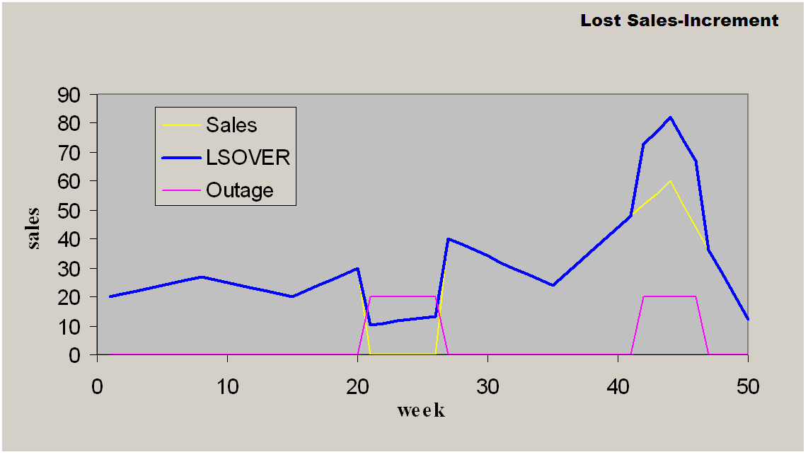
This method increments or decrements the destination measure by the source measure, which is adjusted by the adjustment percentage according to the mask. It is recommended for updating outliers or data gaps when an existing reference measure exists as a default adjustment.
Increment provides the following features:
It is a simple data increment of a given percentage of the reference data to copy from.
It may or may not take outage information (for example, event) as an input to mask the operation.
Has one required parameter, Reference measure to increment by.
Can accept one optional parameter, Ratio of reference to actually increment by.
This method uses the following inputs:
A source measure that can be any measure in the system as long as it has the same intersection as the destination measure.
A reference measure that can be any measure in the system as long as it has the same intersection as the destination measure.
A destination measure that can be any measure in the system as long as it has the same intersection as the source measure.
A mask that is a Boolean measure that has the same intersection as the source and destination measures.
An adjustment percentage.
This method increments or decrements the destination measure by the source measure, which is adjusted by the adjustment percentage according to the mask.
Let:
S(i) is the value in cell (i) of the source measure
R(i) is the value in cell(i) of the reference measure
D(i) is the value in cell (i) of the destination measure
M(i) is the value of cell (i) of the mask
a is an adjustment percentage (can be between (-100%) and (+100%) )
The result of the reduction method is:
D(i) = S(i) + a * R(i) if M(i) is True
D(i) = S(i) if M(i) is False
This is used for canceling the effect of some former preprocessing adjustments.
Clear provides the following features:
Does not take outage information as an input.
May or may not take time series mask (does not have calendar dimension) input to retain results for certain time series.
If time series mask is specified, one duplicated LSOVER measure must be provided in addition to the original LSOVER measure.
IF TimeSeriesMask is provided & TimeSeriesMask = false THEN
LSOVER(t) = LSOVER_REF(t)
LS(t) = LSOVER_REF(t) - SRC(t)
ELSE
LSOVER(t) = 0
LS(t) = 0
A filter removing pricing effects: smoothed=original*(price/maxprice)*(price/maxprice)
LSOVER:LSOVER1, LS:LS1 <-preprocess(SRC:POS, METHODID:mthid, LSTODAY:TODAY1, NPTS:npts, TSMASK_DENSE:tsMask1,PRICE:price.MAX LSOVER_REF:lsoverref1)