Performing Period-End Processing

This chapter provides an overview of period-end processing and discusses how to:

• Summarize forecasts.

• Prorate forecasts.

• Process midperiod forecasts.

• Process period-end forecasts.

Understanding Period-End Processing

You use the Period End Forecast process (DP_CALCFC) to calculate a forecast. This is the business process that you perform at the end of a sales cycle. PeopleSoft Demand Planning also provides an option to make adjustments in the middle of a sales cycle, using the Mid Period Forecast process (DP_FCMIDCALC). The system generates a forecast at each level of a view for each item.

These cycles are recurring business events that are normally driven by the date on which new demand is brought into the forecasting system. Since forecasts are driven by demand, the new data represents a new cycle of forecasting, regardless of the cycle's length. PeopleSoft Demand Planning helps you control forecast parameters, establish forecast cycles, and process forecasts through the cycles.

To perform period-end processing, you:

1. Post new demand.

2. Summarize the forecast.

3. Run period-end processing.

4. Prorate the forecast.

5. Create a summary forecast.

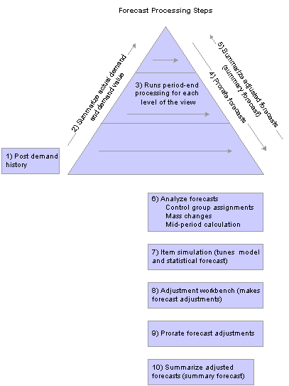
This diagram illustrates the flow of period-end processing:

Importing and loading forecast data from external sources

Forecast calculations take place at step three. But, as part of the forecasting flow, you perform steps one through five. Step five is similar to step two because it arrives at a final summarized forecast. Steps 6 through 10 are optional tuning steps that you perform after the completion of the required steps one through five.

Steps six and seven are looped steps where you analyze the forecast based on various criteria and then simulate the forecast to improve the forecast and forecast error. The steps are a reiterative process that continues until you can is no longer improve the forecast.

You can loop through steps 8, 9, and 10 several times depending on the forecast view level at which you are making adjustments. For example, you could first make adjustments at the lowest level representing collaboration with customers or account managers. You could then override those adjustments at higher levels by sales management and prorate them down through the view. In another example, you could first make adjustments at one of the high levels representing a budget or sales push goals. You could prorate those adjustments down through the view, but then override them at lower levels to represent what the customer anticipates as actual needs.

Note. You can perform midperiod processing as you analyze forecasts. If you incorporate massive changes to items and need to see the effect of those changes, you can run this interim calculation to update the forecasts without moving forward in periods. This affects only those items that are set for recalculation.

Forecast Calculation Process Flows

This section provides flow charts that describe processing during period-end and midperiod processing and discusses:

• General processing.

• Midperiod forecast processing.

• Period-end processing.

• Forecast method determination.

• Moving average processing.

• Post-period processing for each item.

General Processing

This flow chart provides an overview of how the system processes midperiod and period-end forecasts:

General processing

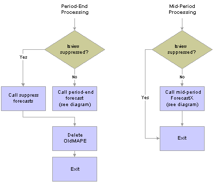
Midperiod Forecast Processing

Midperiod processing is an optional business technique for updating multiple forecast items in a forecast view. This flow chart illustrates midperiod processing:

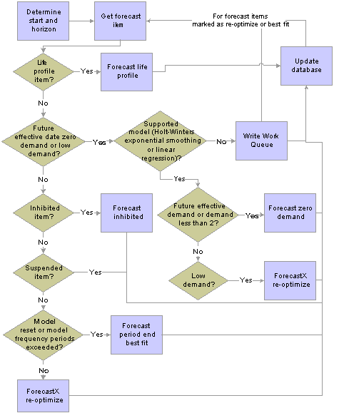
Midperiod forecast processing

Period-End Processing

Period-end processing is a recurring business event that is normally driven by the date on which new demand is brought into the forecasting system. This flow chart illustrates period-end processing:

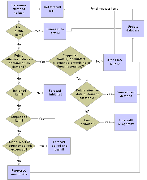
Period-end forecast processing

Forecast Method Determination

A variety of control parameters are available for forecast calculations. Depending on the parameters that are defined for an item, the system determines which forecast method to use. This flow chart illustrates how the system determines the forecast method:

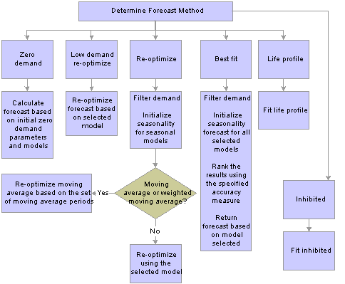
Forecast method determination

Moving Average Calculations

Moving average calculations determine the average of a data series over a specific number of preceding periods. When a new value is added, the system drops the last period from the calculation, so that the specific number of preceding periods remains constant. This flow chart illustrates how the system calculates moving averages:

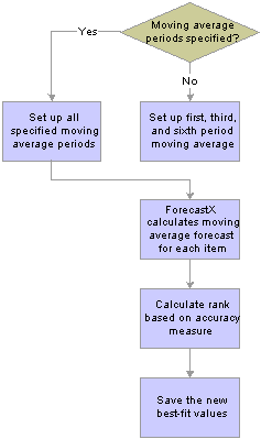
Moving average calculation

Post-Period Processing for Each Item

Post-period processing is when the system populate forecast values for items. This can include statistical, adjusted, and prorated forecast values. This flow chart illustrates how the system processes items at the end of midperiod or period-end processing:

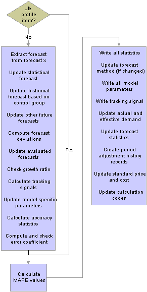
Post-period forecast processing

Period-End Processing Steps

These steps describe the basic forecast calculation steps that you use with period-end processing:

1. Summarize the actual demand by using the Summarization process (DP_SUMMCALC).

   At this point, information is at the lowest level of the view. Summarization rolls up the demand for the selected periods up the view structure from the lowest to the highest level.

   You also use the Summarization process to create a summary forecast toward the end of the process. The summary forecast for an item in a period is equal to the sum of the adjusted forecasts in the same period over all of the item's children (directly related items at the next level down). The system creates a summary forecast for each level except level one.

   If you are performing period-end processing, the new demand data is normally for the current first forecast period. This period becomes the latest historical period after the period-end processing is complete.

   To summarize demand:

   1. Create a summarization specification that provides more control over summarization parameters.

      This includes levels, periods, or both for summarization. Use the specification to run the Summarization process. Be sure to select the Create Missing Groups and Delete Groups without Details check boxes and select Actual Demand and Demand Value as the roll-up options.

   2. Run the summarization by using the Summarize option.

      This process summarizes the data for the options that are selected in the specification. Using the options in step a, the process creates any parent items that do not currently exist so that the demand can be summarized to those levels. The system removes parent items without children to keep the view as clean and uncluttered as possible.

   3. Review the Work Queue Workbench for added alerts.

      Select either the Review Added Group Item or Review Auto Added Item message to view in the Work Queue. Also check for alerts that are generated during the rollup. These alerts relate to new items that are normally added at upper levels of the view. Review the items to ensure that certain data elements are correct, such as the units of measure and the next-level conversion factors.

   4. Verify that actual demand is summarized correctly and the next-level conversion factors are correct.

      Also verify that the description, caption, unit of measure (UOM), UOM conversion factors, standard price and cost are set up correctly. Make sure that the forecast effective date, model, and model components are set correctly for future-dated items. These are items that do not have demand until a future date.

   5. Correct the alerts and, if necessary, rerun the Summarization process.

2. Create a period-end forecast using the Period End Forecast option.

   You use this option when the sales cycle is complete and you are ready to start on the next forecast cycle. During period-end processing, the system moves the forecast forward one period and updates the demand. To access the options, select Process Forecasts, Calculation.

   When calculating a forecast, the system can make adjustments for promotions, filter abnormal demand, and generate a statistical forecast for each item at each level of the view. The system calculates the forecast at each level so that you can compare the aggregate, or summary, and statistical forecasts.

   Midperiod processing is an optional technique that you use to update forecast items in a forecast view that are set for the system to reforecast. You normally use this process after making mass changes to items, such as changing control group parameters. You use period-end processing to complete a forecast cycle. In this case, the system advances the forecast start period by one period, extending the forecast by one period as well.

   The view determines the number of future forecast periods that the system calculates, which is typically two years. You can recreate a forecast as many times as you need to during a period. However, only those items that are set to reforecast actually are updated by the midperiod process calculation. You might use simulation to recreate a forecast for an item regardless of whether the item is set for reforecasting.

   Items that are associated with an active life profile follow the same process for the depromotion of events and filtering of demand. The expected life to date and demand to date are then recalculated.

   After generating the forecast:

   1. Review poorly forecasted items by using the Analyze Forecast feature.

      The review lists items in descending sequence, based on the error ratio. This ratio is a calculated result of the statistical forecast deviation divided by the demand average. This provides a relative error so that the system can sort those items with high error and lower demand to the top of the list. Items with low error and high demand are at the bottom of the list.

      Reviewing those items that have a high relative error, or error ratio, results in a more significant impact if you can reduce the forecast error. You should also consider sorting the list by demand average so that you can make possible improvements to high-volume items. Also consider sorting by standard cost, because improvements to the forecast for those items can result in a significant impact to the bottom line in safety stock reductions.

      Insufficient history, unfiltered events in the demand, or promotions, among other factors, might cause poor results. You can make adjustments to the demand, add control groups, or add seasonality groups to improve the results.

      Another situation that causes poor results is when an item assumes a particular model, but that model is no longer a good fit. This might occur when the model change frequency prevents the item from choosing another model. Poor results can occur if you do not have enough history (fewer than two years) for an item that is obviously a seasonal item. You might associate it with a seasonality group that is set up for the product group to which the item belongs.

      Another example of poor results is when a new product launch causes extremely high demand in the earliest demand period. You might eliminate the launch data by shortening the demand horizon or by maintaining the demand.

   2. Review the Work Queue for alerts that are created during the forecast generation.

      Concentrate on alerts that are generated by the period-end forecast generation. Make adjustments as necessary and use simulation routines to correct problems.

   3. Tune the forecast.

      The statistical forecast that the system calculates is the starting point for management review and input. It is management's responsibility to apply overrides that reflect promotions that are not already adjusted for, new product introductions, competitive product activity, and other market activity.

      This step may also include investigating and correcting notifiable events, such as resetting the model, and Work Queue alerts, such as filtering outliers, that have been logged to the Work Queue during the previous procedures. Management makes adjustments more often at higher levels in the view because they have a more general idea of required adjustments. You can prorate these adjustments down through the view as described in the next step.

      Other techniques of tuning the forecast include customer or account manager collaboration. This might include making forecast adjustments at lower levels in the view which may overwrite or augment existing adjustments. You summarize those adjustments up through the view so that you can review a comparison of the total effect.

3. Prorate the forecast.

   The Proration process (DP_PROCALC) allocates the item (group) forecasts for each future period. It makes the allocation by period to the forecasts of the related items (children) at the next lower level. The allocation is on a prorated basis based on the future forecasts of the children. The effect is to make the aggregate forecast of children equal to the group forecast. The system can base the proration on the statistical forecast or the prorated forecast in a normal forecast view. You can prorate dynamic views on the basis of the adjusted forecast.

   The prorated forecast tends to be more accurate than the statistical forecast. The Proration process factors the group forecast down one level at a time to make the sum of the item forecast equal to the aggregate forecast.

   To prorate a forecast:

   1. Create a proration specification.

      Verify that the proration specification is set to include processing parameters that you want. Prorate the view from the highest proration level to level one. The highest proration level is normally the highest level in the view, but this may not be so if there are summary levels (one or more) at the top of the view. Summary levels are those that group all items into only a few group items and represent a summary review level and not forecast patterns that you want for proration.

   2. Prorate the forecast by using the Prorate option.

      See Prorating Forecasts.

   3. Balance the view.

      Balancing ensures that individual forecasts are consistent with (equal to) higher-level forecasts. At this point, it is also necessary to balance the view. To do this, you must run the Summarization process again from the bottom (level one) to the top of the view to create a summary forecast.

   4. Review the Work Queue for proration errors and alerts.

      These relate to things like abnormal proration ratios, missing children, and the like. Proration errors can be serious and need to be reviewed carefully. Make adjustments as necessary and run simulation to correct the problem.

   5. Make adjustments and rebalance the view.

      Apply management forecast adjustments to reflect market influences that are not reflected in the forecast. This can easily include adding items that are to be introduced at some time in the future. Make sure that the forecast effective date, model, and model components are set correctly for these items. You must prorate and summarize the forecast again to bring all the numbers back into balance.

   6. Rerun the Proration process after making adjustments.

4. Run the Summarization process a final time from the bottom to top of the view.

   See Summarizing Forecasts.

   1. Select the Summary Forecast rollup option on the summarize specification Rollup Options page. All other items should be left at their default values.

   2. Check the Work Queue for alerts that are generated during the process run. There should not be any alerts.

Summarizing Forecasts

This section provides an overview of summarization and discusses how to:

• Define summarization specification levels, periods, and groups.

• Define summarization specification roll-up parameters.

• Run forecast summarization.

Understanding Summarization

Summarizing a forecast accumulates data and updates it from a lower level in the forecast view hierarchy to higher levels. The starting level and higher levels are updated based on the number of levels that you select to process. Usually the starting level is the level at which demand data is brought into the system; this is most often the lowest level in the forecast structure. The actual sets of accumulated data are controlled by the roll-up options that you define.

This diagram displays the detailed sales history for peanuts that is set up to be summarized into several levels of aggregation:

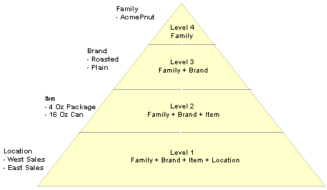
Example of a forecast view structured for summarization

So, for example, the base data might contain the details of sales for each stockkeeping unit at West and East Sales locations. This can be summarized first into sales of the item across all locations. Further levels of summarization show the data by roasted or plain brands, and, at level four, the AcmePnut family.

Two records in PeopleTools are used to store the forecast items data. One record, DP_FCITEMS, contains all non-time-phased information about the item and how it is processed. The other record, DP_FCITEMDATA, contains all time-phased data that the system uses and generates when producing forecasts. Level two to four quantities would be derived during the summarization process. The next table shows historical actual demand data that might be stored in the record DP_FCITEMDATA table for level one items from the previous examples:

To roll up quantities, you use the Summarization process. The next diagram describes how the system applies values from the DP_FCITEMDATA record fields to build the four levels of a view:

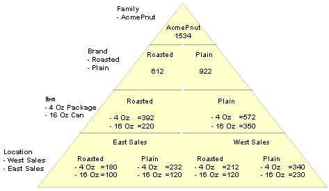
Rolling up values in a forecast view during summarization

Note. It is important to match the selected periods with the type of data that you are rolling up. For example, if you only hold demand for past periods, you should only select the appropriate period range. Normally, the first summarization requirement in period-end processing is for demand, and PeopleSoft recommends that you do not attempt to mix a roll-up of demand-related data with another type of roll-up unless it applies to same period range at the same time.

In most cases, you can leave the period settings at their default values, which summarizes demand across the entire horizon. The default values ensure that demand data that is posted as corrections to historical periods is processed and that an updated forecast is generated to reflect those corrections.

In addition to rolling up demand and forecast data, summarization can also roll up historical forecasts, standard cost, standard price, demand, and numeric user-defined data sets. You can also update user-defined fields, but since some of these are nonnumeric, the system uses the value of the last child forecast item to replace the value at the next level.

Pages Used to Summarize Forecasts

Defining Summarization Specification Levels, Periods, and Groups

Access the Summarization Specification page.

Use the RESET item when Demand in period changes by more than option to have the system set forecast items to have their forecast models reset if there are fluctuations that fall outside this percentage. When you define a percentage, items with a percentage of change that is greater than the one that you enter are automatically included when you run the next Update process. The default value is 5.

Levels to Process

Define which items you want to include in the summarization process. The system bases the summarization on a forecast view, so you can limit the items to certain levels in the view or include all items at all levels.

Period Control

Defines periods and years for the summarization. The fields use default values that include a range from the first forecast period to the last forecast period. The Update From field values appear by default from the view's forecast start year and period. The update-to period and year appear by default from the view's configuration future periods. When you select Actual Demand on the Rollup Options page, the system changes the range to start at the first historical period (last demand).

To update the Update From or To fields, type over the existing values. The period and year of the selections appear in the Last Demand, First Forecast, and Last Forecast fields.

When performing period-end processing, you normally summarize from the level at which new actual demand was imported (level one) up to the highest level in the hierarchy. Also, the number of periods that are being updated significantly impacts performance. If you are only updating demand, then select only the period range in which the demand has changed at the lower level. This might include all historical periods, but not future periods beyond the current period.

If you have not entered demand for future periods (the normal situation), then you should use the first forecast period as the update-to period and year. Similarly, if you intend to roll up future forecasts or summarized forecasts, also consider the appropriate period range.

Group Create/Delete Control

Define how the system processes parent items. You should select both check boxes so that the system creates parent or group items as needed. Also, the system deletes group items that are no longer needed because supporting child items are removed.

Defining Summarization Specification Roll-Up Options

Access the Rollup Options page.

Use this page to define which fields of data you want the system to use when summarizing a forecast. For example, suppose you are at the start of period-end processing and want to roll up actual demand, select the Summarize check box for the Actual Demand field. At the minimum, when summarizing a forecast, the system calculates a summary forecast for the levels that you select on the Summarization Levels page.

Click Select All to include all fields of data. Click Clear All to clear the selections.

Click Apply to update this page with the options you selected. You can roll up data for these fields:

Running Forecast Summarization

Access the Summarize page.

Select which summarization specification controls the Summarization process.

Use the Adjustment Reason Code field to select a user-defined reason that the system uses to track changes that are made to demand history. You use the codes to identify recurring adjustments. You define reason codes using the Adjustment Reason Code page. To access the page, select Define Forecast Elements, Adjustment Reasons. Enter an Adjustment Comment to explain the adjustment.

See Also

Defining Summarization Specification Levels, Periods, and Groups

Prorating Forecasts

This section provides an overview of proration and describes how to:

• Define proration specification levels, periods, and thresholds.

• Run forecast proration.

Understanding Proration

After you make adjustments, proration takes the aggregate item forecast at each level and sets the forecast of the items at the next level down equal to the aggregate group forecast. This means that the higher-level forecasts, which are generally more accurate, and any adjustments made at higher levels, are passed down the view hierarchy.

The system calculates the allocation weights period-by-period on the basis of the statistical or prorated future forecast. Dynamic views allow the additional basis of the adjusted forecast. The advantage of using allocation weights over fixed proportions or an historical mix is that it reflects an evolving product mix.

During proration, the system processes forecast views from top to bottom. This means that the higher-level forecasts, which are generally more accurate, and any adjustments made at higher levels are passed down the view hierarchy.

For example, products 1, 2, and 3 are all part of the same product group, Brand X. The system generates the statistical forecast and aggregate forecast:

During proration, the system calculates a proration factor that is equal to the ratio between the group forecast and the sum of the forecasts of the children. This calculation is performed period by period. In the next tables, the system calculates these factors:

Period 1: 176 ÷ 160 = 1.1

Period 2: 207 ÷ 180 = 1.15

This factor is applied to the statistical forecast for each child in order to produce the prorated forecast.

The period one prorated forecast is:

The period two prorated forecast is:

Pages Used to Prorate Forecasts

Defining Proration Specification Levels, Periods, and Thresholds

Access the Proration Specification page.

Levels to Process

Define which items you want to include in the proration process. The system bases the proration on a forecast view, so you can limit the items to certain levels in the view or include all items at all levels.

Period Control

Specify the periods within which proration is to occur. The fields appear with initial default values that include a range from the first historical period to the last future period. The Update From field values appear by default from the view's forecast start year and period. The update To period and year appear by default from the view's configuration future periods.

Proration Threshold Ratios

Define threshold ratio boundaries. Occasionally, the Proration process creates proration ratios that result in unreasonable prorated forecasts. The system uses the values that you enter as lower and upper bounds in ratio reasonableness checks. The system generates alerts in the Work Queue for items with ratios that are outside the limits.

Proration Basis

Specify the basis for how the system prorates an adjusted forecast. Dynamic views have three options: Statistical, Prorated, or Adjusted, with Adjusted as the default value. All other views use Statistical and Prorated as available values, with Prorated as the default value. You define the default value for this group box by using the Adjustment Basis field on the User Preferences page.

Defining Proration Options

Access the Prorate Options page.

Use this page to define which fields of data you want the system to use when prorating a forecast. Select the Prorate check box for the forecast fields that you want to prorate during period-end and midperiod processing.

Running Forecast Proration

Access the Proration page.

Use this page to select which proration specification controls the Proration process. Use the Adjustment Reason Code field to select a user-defined reason that the system uses to track changes that are made to demand history. You use the codes to identify recurring adjustments. You define reason codes using the Adjustment Reason Code page. To access the page, select Define Forecast Elements, Adjustment Reasons. Enter an Adjustment Comment to explain the adjustment.

See Also

Defining Proration Specification Levels, Periods, and Thresholds

Processing Midperiod Forecasts

This section provides an overview midperiod processing and discusses how to run midperiod forecasts.

Understanding Midperiod Processing

Midperiod processing is an optional technique for updating multiple forecast items in a forecast view. For example, if you have made mass changes for items, adjusted item quantities, or changed model controls, you can use midperiod processing to recalculate the forecasts for those items.

Midperiod processing might include:

• Reviewing and revising control group settings.

  Set items for processing to Best Fit or Reoptimize by using the Model Control page when you maintain forecast items.

  Some items may already be ready for processing because of one of the following actions:

  • Changes are made to the item's control group.

  • Actual or adjusted demand is posted or maintained at level one.

  • Actual or adjusted demand changed by more than a user-specified threshold (defaults to 5 percent).

  • The forecast is determined to have a high error or be biased.

• Recalculating seasonality groups.

  This is necessary if you make changes to the seasonality profile, such as adding a contributor.

• Applying forecast adjustments to include market influences that are not reflected in the forecast.

  For example, adding items that are to be introduced at some time in the future or introducing a new promotion. Make sure that the forecast effective date, model, and model components are set correctly for these items.

• Maintaining event data and reapply event weights, if needed.

• Reviewing the Work Queue for alerts from the previous period-end processing, making item adjustments, and running the Simulation process if necessary.

• Finalizing tuning adjustments, such as making sure cost and price information is accurate.

After fine tuning the forecast, you can use the Mid Period Forecast option to perform midperiod processing before going on to period-end processing.

Page Used to Process Midperiod Forecasts

Running Midperiod Forecasts

Access the Mid Period Forecast page.

Create a forecast for midperiod processing.

Processing Period-End Forecasts

This section provides an overview of period-end processing and describes how to run period-end processes.

Understanding Period-End Processing

Period-end processing is when you roll forecast periods forward one period. During processing, the system optimizes all items at the minimum. For items that you select, you can also perform best-fit processing. The system might also select items on which to perform best-fit processing. Period-end procedures are performed once per view

When you are ready to advance to the next period, make sure that you have all demand for future periods, have transferred the demand and summarized it. Then you can run the forecast calculation in period-end mode.

Page Used to Process Period-End Forecasts

Running Period-End Forecasts

Access the Period End Forecast page.

Select a forecast view against which to perform period-end processing.