Defining Forecasting Rules
This chapter covers the following topics:
- Overview – Forecasting Rules
- Defining Usage, Shipments, or Returns Based Forecasting Rules
- Population-Based Forecast Rules
- Setting Up Install Base, Failure, Return, and Retirement Rates
- Defining Product Population Based Forecast Rule Parameters
- Dual Output Levels
- Defining Forecast Rule Horizon Details
- Available Forecasting Methods
- Setting Forecasting Method Basic Parameters
- Setting Forecasting Method Advanced Parameters
- Setting the Intermittent Demand Inventory Item Attribute
- Associating Forecasting Rules with Items
- Setting Up Lifetime Buy Functionality
Overview – Forecasting Rules
You specify forecast rules to determine the history source and the forecast methods to use when generating the spare part forecasts. All parts in the scope of the plan associated with the appropriate forecast rule are forecast.
You specify the forecast method and the data stream basis of forecast calculations in the Forecast Rules window. This form consists of a header region and three tabs:
-
Usage / Shipment / Return Forecast
-
Product Population Forecast
-
Horizon Details
This chapter explains how to:
-
Define usage, shipment. or returns-based forecasting rules.
-
Assign the forecast method and other parameters.
-
Define the basis for calculating the forecast.
-
-
Define population-based forecasting rules.
-
Define install base population, failure rate, and retirement rate parameters.
-
Assign the forecast method and other parameters.
-
Define the basis for calculating the forecast.
Note: It is possible to set up both usage based and population based forecasts for the same item. See Dual Output Levels.
-
-
Associating forecast rules with items.
-
Assign forecast rules to items
-
Update or change the forecast rule assigned to these items.
-
Defining Usage, Shipments, or Returns Based Forecasting Rules
You use the Forecast Rules window to assign the forecast method and define the basis for calculating the forecast.
To define usage, shipment, or returns-based forecast rules
-
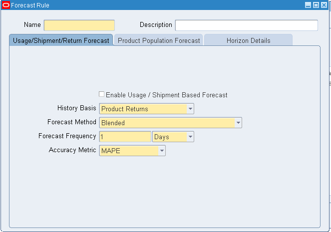
From the Service Supply Chain Planner responsibility, navigate to the Forecasting Rules window.
Setup > Forecast Rules Forecasting Rules – Usage / Shipment / Return Forecast tab
The Forecast Rule window appears, with the Usage/Shipment/Return Forecast tab selected.
-
Define the forecast rule name and description.
-
Select the Usage/Shipment/Return Forecast tab.
-
To enable Usage and Shipment based forecasting, select the Usage/Shipment/Return Forecast check box.
-
Define the forecast rule parameters. For a description of these parameters, see the table that immediately follows this procedure.
-
Select History Basis from the LOV. See Inline Forecasting Concepts.
Note: Inline forecasting generates forecasts for an item at either the zone level or the organization level.
-
If the history stream is based on field technicians’ usage, the forecast is at the zone level.
-
If the history stream is based on shipment or usage (component issue) at the internal repair depot organization, the forecast is at the organization ship from level.
-
-
Select the forecast method from the LOV. See Available Forecasting Methods.
-
Set the Forecast Frequency.
-
Choose one of the following accuracy metrics from the LOV.
-
Mean Absolute Percentage Error (MAPE)
-
Mean Absolute Deviation (MAD)
-
-
-
(Optional) Change the Forecast Method parameter default values. See Setting Forecasting Method Basic Parameters.
-
Click Save.
-
Proceed to Defining the Forecast Rule Horizon Details.
Forecasting Rules – Usage/Shipment/Return Forecast tab parameters:Forecasting RuleParameters Field Description Validation Default Value (Header) Name The Forecast Rule name entered here calls the forecast rule. (Header) Description Optional. You can enter an extended definition for the forecast rule. Enable Usage / Shipment Based Forecast Select the check box to enable forecasts based on Usage and Shipment data streams. Not Selected History Basis This field lists collected data streams of usage and shipment history from returns of products and service parts. LOV, history data streams None Forecast Method Select a supported forecast method.
See Inline Forecasting Overview.LOV, supported forecast methods None Forecasting Frequency Planning records retain the latest forecast date for each item and group combination. Planning regenerates forecasts based on the frequency specified here. Number and bucket size (days, weeks, or periods) Accuracy Metric Select the calculation method to measure forecast accuracy. Mean absolute deviation (MAD), or Mean absolute percent of error (MAPE) MAPE
Population-Based Forecast Rules
This alternative approach to calculating forecasts is often used when history data is insufficient to reliably calculate a forecast.
Decision Diagrams for Selecting Population-Based Forecast Rule Parameters
When suitable data is available, you can choose to allow the system to calculate factors used in the population based projections. When data is not available, you enter estimates for these values based on your experience. The following flow diagrams illustrate the decision process in selecting elements of population based forecasting:
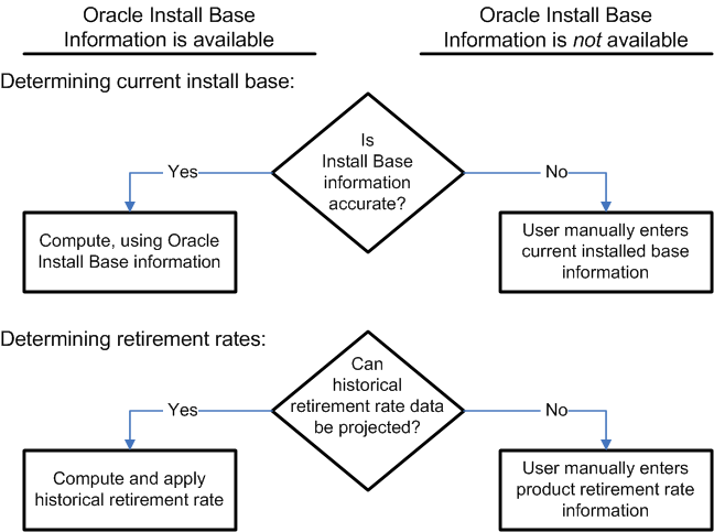
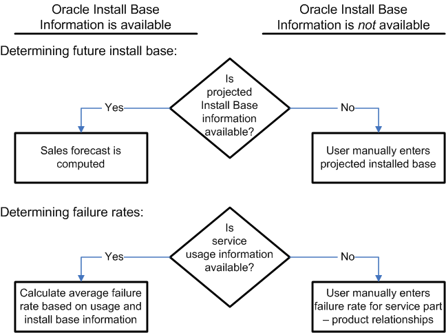
As seen in the previous diagrams, if information from Oracle Installed Base is not available, you provide the relevant data needed to calculate projected demand. When the relevant data is not provided, the following assumptions are made, and appropriate warning messages are provided in the log file:
| Oracle Installed base available | Oracle Install Base not available | |
|---|---|---|
| Current installed base | Manual entry (but not provided) – Assume zero | Manual entry (but not provided) – Assume zero |
| Retirement rate | Manual entry (but not provided) – Assume zero | Manual entry (but not provided) – Assume zero |
| Projected installed base | Calculated, but sales order history is not available – Assume zero and provide a warning in the log file | Manual entry (but not provided) – Assume zero and provide a warning in the log file |
| Failure rate | Manual entry (but not provided) – Assume zero and provide a warning | Manual entry (but not provided) – Assume zero and provide a warning |
Product Population Based Forecasting Rule Parameters
This section describes how to manually enter the following Forecast Rule parameters for Product Population based forecasts:
-
Failure Rate and Return Rate for the combination of product and service part, as determined by the service item relationship.
Users typically base returns forecasts of newly introduced products on failure rate forecasts. For existing products, you might prefer to employ usage-based or shipment-based forecasts. In such cases, to avoid doubling demand from the failures of existing products, ensure that failure rates and return rates are not entered for existing products in the forecasting rule.
-
Product retirement rate to decrement the installed base population.
-
Current installed base needs to be entered when information from Oracle Install Base is not available.
The entries are global (or organization independent) in nature.
Setting Up Install Base, Failure, Return, and Retirement Rates
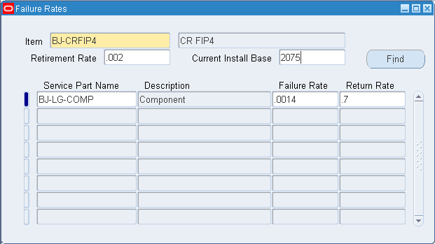
The Failure Rate window, available from the Setup menu, captures the average failure rates, return rates, retirement rates, and currently installed base population information.
-
You cannot add any new product and service part relationships in this window. The service item relationship is based on collected information.
-
Organization is not part of the find criteria, because this information is independent of organization.
-
From the Service Supply Chain Planner responsibility, navigate to the Failure Rates window.
Setup > Failure Rates
-
In the header region, select the product. The scope of the items is limited to items that are parent items in the service relationship.
-
Click Find.
The system populates the Product region of the Failure Rate form according to the find criteria.
Note: You can select a new product at the header level, if needed.
To Set the Retirement Rate and the Current Install Base
-
You can manually enter the retirement rate for the selected product, in percent per time bucket.
-
You can also manually enter the quantity of the selected product that represents the number of units that are currently installed.
To Set the Failure Rate and the Return Rate
-
when you select a product, the Service Part name region is populated with all the relevant service parts with which service relationships are established.
Note: Query functionality (F11 and Ctrl F11) is available in the Service Part Name region.
-
Select a service part.
-
Enter the average failure rate and average return rate for the selected service part, in percent per time bucket.
-
Click Save.
Defining Product Population Based Forecast Rule Parameters
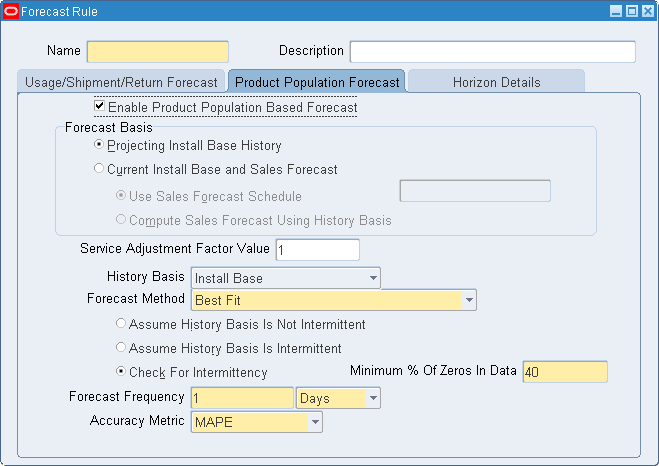
You specify Forecasting Rule parameters for population based forecasting in the Product Population Forecast tab of the Forecasting Rule window. The parameters for non-product population-based forecasts appear under the Usage/Shipment/Return Forecast tab. See Defining Usage Based Forecast Rules.
To specify product population-based forecasting rule parameters
-
From the Service Supply Chain Planner responsibility, navigate to the Forecast Rule form.
Setup > Forecast Rules
-
Select the Product Population Forecast tab.
-
Define the forecast rule name and description.
-
Select the Product Population Forecast tab.
To Define Forecast Rule Parameters
-
To enable forecasts based on install base population and failure rates, select the Enable Product Population Based Forecast check box.
-
Choose one of the following forecast basis radio buttons.:
-
Projecting Install Base History
-
Current Install Base & Sales Forecast.
If you select the Projecting Install Base History radio button:
-
The Use Sales Forecast Schedule and Compute Sales Forecast Using History radio buttons are disabled.
-
The History Basis is automatically set to Install Base.
If you select the Current Install Base & Sales Forecast radio button, the following two radio buttons are enabled:
-
Use Sales Forecast Schedule (or upload a flat file).
-
Compute the Sales Forecast Using History.
If you select Use Sales Forecast Schedule, and you want to upload a flat file, you can then point to a Demand Schedule for the Sales Forecast. Then select the flat file to be uploaded from the network. In the case of a flat file upload, the file is collected and presented as a schedule.
The control file for the flat file loading of sales forecast is as follows:
Item Quantity Start Date End Date UOM Note: You must load the data in the same bucket as defined in the Forecasting tab of plan options.
-
-
If you select the Compute the Sales Forecast Using History radio button, the system computes the sales forecast. In the History Basis field choose either Usage or Shipment from the list of values.
-
(Optional) Specify the Service Adjustment Factor value in the range of zero to one. Because not all product sales necessarily translate into a service contract, you can use this factor to adjust the sales forecast to account for your estimated service market share.
-
Select the forecast method from the LOV. The forecast method applies to either the install base forecast or sales forecast, depending on previous selections. See Available Forecasting Methods.
-
(Optional) Change the forecast method parameter default values. See Setting Forecasting Method Basic Parameters.
-
Select one of the following radio buttons to indicate whether to use forecasting methods designed for intermittent data history:
-
Assume History Basis is Not Intermittent
-
Assume History Basis is Intermittent
-
Check For Intermittency
If you select the Check for Intermittency radio button, the Minimum % Of Zeros in Data field is enabled. Enter the threshold value..
-
-
Set the forecast frequency.
-
Choose an accuracy metric from the LOV.
-
MAPE
-
MAD
-
-
Click Save.
-
Proceed to Defining the Forecast Rule Horizon Details
Forecasting Rules – Product Population Forecast tab Parameters:Forecasting RuleParameters Field Description Validation Default Value Enable Product Population Based Forecast Select to enable forecasts based on install base population data and failure rates. Not Selected Forecast Basis – Projecting Install Base History Select to create this forecast by projecting the patterns existing in the Install Base History data (only). Radio button Forecast Basis – Current Install Base & Sales Forecast Select to create this forecast based on the current Install Base history data and sales forecasts. The sales forecast can either be available as a demand schedule, or can be computed in the system. Radio button Use Sales Forecast Schedule If the Forecast Basis is Current Install Base & Sales Forecast, select this radio button to use a sales forecast schedule. This radio button enables the LOV for selecting the schedule. Radio button, LOV Compute Sales Forecast Using History If the Forecast Basis is Current Install Base & Sales Forecast, select this radio button to compute the sales forecast based on history. Radio button Service Adjustment Factor Value * The estimated proportion of sold products that are contracted for service. Number, within range zero to one History Basis This field lists collected data streams of usage and shipment history from returns of products and service parts. LOV, data streams Forecast Method Select a supported forecast method. See Inline Forecasting Concepts. LOV, supported forecast methods None Forecasting Frequency Planning retains the latest forecast date for each item and group combination. Planning regenerates forecasts based on the frequency specified here. Number and bucket size (days, weeks, or periods) Accuracy Metric Select the calculation method to measure forecast accuracy. MAD or MAPE MAPE * The Service Adjustment Factor Value is a number in the range of zero to one. Because not all product sales necessarily translate into a service contract, you can use this factor to adjust the sales forecast to provide an estimate of your service market share.
Dual Output Levels
For a given item, it is possible to define output level information for both:
-
Usage or shipment based forecast
-
Product population-based forecast.
This functionality supports the following typical scenario:
You want to use usage-based forecasting for spare parts demand due to established product populations, for which service part usage histories are available, and use failure rate forecasting for new product populations, for which no service part usage histories are available.
If both usage-related and product population-related parameters are defined, and they overlap each other, then the numbers are accumulated to determine the final forecast. Because the levels of output of usage forecasts and product population-based forecast could be different, the accumulation is done at the organization level after distribution of the forecasts.
Dual Output Level Example
It is possible to set up both usage-based and population-based forecasts for the same item. The example describes a scenario where the correct strategy is to enable the failure rate and return rates for only newly introduced products.
-
Cartridge x is used in Printer A and Printer B.
-
The Cartridge x usage-based forecast (total for Printer A and Printer B) is 100 units per month.
-
Printer C is introduced to the market, and uses Cartridge x as well.
-
Due to the introduction of Printer C, usage of Cartridge x is expected to increase by 25 per month.
-
Service part and product relationships are set up for Cartridge x and all three of the printers (A, B, & C).
-
Printers A, B, & C are selected in the Find window to populate the Product region of the Failure Rate form.
-
In the Service Part region, the Cartridge x Service enabled for Product check box is selected for all three printers.
Inaccurate Result: The total forecast for Cartridge x is about 225 per month. This is inaccurate, due to double counting. In this example, 100 cartridges from the usage-based forecast for Printers A and B, plus about 125 cartridges from the population-based forecast that was set up here accumulate to about 225 cartridges.
The correct approach is to enable the failure rate and return rate for only the new product (Printer C). To correct this setup, deselect the Service enabled for Product check boxes for Printer A and Printer B.
Correct Result: If only Printer C is enabled for failure rate and return rate, then the total forecast for Cartridge x = 100 (usage-based) + 25 (product population-based from Printer C) = 125 per month.
Defining Forecast Rule Horizon Details
To define forecast rule horizon details
-
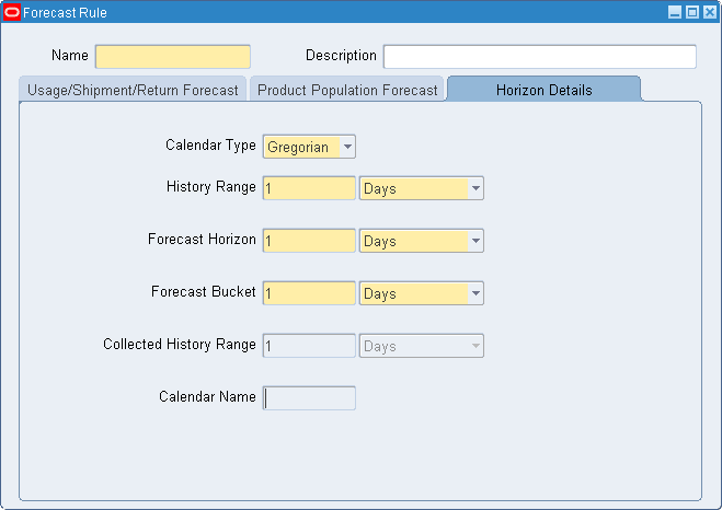
Select the Horizon Details tab.
-
Select the calendar type from the LOV.
-
Gregorian
-
Manufacturing
-
-
Complete the parameters. For a description of the parameters, see the table that immediately follows this procedure.
-
Click Save.
Forecast Rules - Horizon Details tab ParametersForecasting RuleParameters - Horizon Details Field Description Value UOM Default Value Default UOM Calendar Type Defines the calendar type to be applied 1 – Gregorian
2 – ManufacturingNA 2 – Manufacturing NA History Range Historical periods of data to be considered * Positive integer Manufacturing: Days, Weeks, Periods 1 Month Forecast Horizon Future periods for which forecast is generated Positive integer Manufacturing: Days, Weeks, Periods
Gregorian: Months, Quarters, Years1 Month Forecast Bucket Size of time bucket for generated forecasts, and as well as the history Positive integer Manufacturing: Days, Weeks, Periods
Gregorian: Months, Quarters, Years1 Month Collected History Range This noneditable field displays the maximum value for the ‘History Range’ setting. ** Calendar Name When Calendar Type is Manufacturing, this noneditable field displays the Calendar name . * When the user specifies multiple forecast methods for an item, the History Range specified here applies to all methods. Each method, however, can be based on a different collection stream, for example, usage-based forecasting for parts where usage history is available, and product population-based forecasting where the part usage history is not available.
** The Collected History Range is the shortest of all the ranges of the individual streams that are being used.
Note: If the Manufacturing calendar is specified, then the forecasting engine uses the calendar specified in the profile Calendar reference for bucketing. In the absence of this profile setting, the forecasting engine uses the Manufacturing calendar for the organization that owns the plan.
Available Forecasting Methods
The available forecast methods are:
-
Blended
-
Single Exponential Smoothing
-
Double Exponential Smoothing (Holt)
-
Integrated Causal Exponential Smoothing (Modified Winters)
-
Regression with seasonal causal factors
-
Multiplicative Monte Carlo regression with seasonal causal factors
-
Croston for intermittent data
-
Regression with seasonal causal for intermittent data
-
Multiplicative Monte Carlo regression with seasonal causal factors for intermittent data
The Blended forecast is a Bayesian information criterion weighted combination of several methods. For non intermittent data, the engine uses methods 2 through 6. For intermittent data, the engine uses methods 7 through 9.
During SPP setup, each forecasting method is seeded with a set of instance-level default parameter values. To set the default values, see Setting Forecasting Method Advanced Parameters.
Setting Forecasting Method Basic Parameters
You can use the following procedures to specify forecast parameters for each forecasting method.
To set basic parameters
-
From the Service Supply Chain Planner responsibility, navigate to the Forecast Parameters window.
Setup > Advanced Forecasting Parameters
The Forecast Parameters window opens to the Basic tab.
-
In the Parameters region, select one of the following radio buttons:
-
Determine Optimal Constants Automatically
-
Use Values Below
If you chose Determine Optimal Constants Automatically, you can not set the following parameter values:
-
Level Coefficient (Alpha)
-
Trend Coefficient (Gamma)
-
-
If you chose the Use Values Below radio button, you can specify parameter values relevant to the selected forecasting method. The following tables describe the basic forecast parameters for each supported forecast method.
Simple moving average Parameter Default Value Validation / LOV Comments Moving Average Interval 3 Integer,
Minimum value = 2Simple exponential smoothing Parameter Default Value Validation / LOV Comments Alpha (smoothing constant for demand level) None Valid values in the range from 0 to 1. If this parameter is omitted, the forecast engine computes this smoothing constant value. Holt, and Croston for intermittent history data Parameter Default Value Validation / LOV Comments Alpha (smoothing constant for demand level) None Valid values in the range from 0 to 1. If this parameter is omitted, the forecast engine computes this smoothing constant value. Gamma (smoothing constant for trend) None Valid values in the range from 0 to 1 If this parameter is omitted, the forecast engine computes this smoothing constant value. Modified Winters (integrated causal exponential smoothing) Parameter Default Value Validation / LOV Comments Alpha (smoothing constant for demand level) None Valid values in the range from 0 to 1. If this parameter is omitted, the forecast engine computes this smoothing constant value. Gamma (smoothing constant for trend) None Valid values in the range from 0 to 1 If this parameter is omitted, the forecast engine computes this smoothing constant value. Seasonal Period * Year Week, Year Method
-
Regression with seasonal causal
-
Multiplicative Monte Carlo regression with seasonal causal
-
Regression with seasonal causal for intermittent data, and
-
Multiplicative Monte Carlo Regression with season causal for intermittent data
Parameter Default Value Validation / LOV Comments Seasonal Period * Year Week, Year Note: * Seasonal Periods
-
If the forecast uses the Manufacturing calendar, then select week or year.
-
If the forecast uses the Gregorian calendar, then select year.
-
The selected bucket size value should be at a higher (more aggregate) level than the forecasting bucket size. For example, if the forecast is calculated in monthly buckets using the Gregorian calendar, then the only eligible value for seasonal period is year, which is at a higher level of aggregation than monthly buckets.
-
If the seasonal period value is omitted, or an invalid value is specified, then the assumed value is year.
Blended Parameters
If you know the data is non intermittent, then you can specify parameters for methods:
-
2. Single Exponential Smoothing
-
3. Double Exponential Smoothing (Holt)
-
4. Integrated Causal Exponential Smoothing (Modified Winters)
-
5. Regression with seasonal causal factors
-
6. Multiplicative Monte Carlo regression with seasonal causal factors
If you know the data is intermittent, then you can specify parameters for methods:
-
7. Croston for intermittent data
-
8. Regression with seasonal causal for intermittent data
-
9. Multiplicative Monte Carlo regression with seasonal causal factors for intermittent data
Preprocessing
The following basic preprocessing controls are available for adjusting the data:
Parameter Default Value Validation / LOV Ignore Leading Zeros No, if intermittent
Yes, if non intermittentCheck box Fill Missing Values LOV
Fill Missing Values with Zeros, Fill Missing Values with Linear Interpolation, OmitCorrect Gross Outliers Yes (check box selected) Check box -
Setting Forecasting Method Advanced Parameters
Setting the Advanced Parameters provides fine control of the forecasting process.
To set advanced parameters
-
From the Service Supply Chain Planner responsibility, navigate to the Forecast Parameters window.
Setup > Advanced Forecasting Parameters
The Forecast Parameters window opens to the Basic tab.
-
Select the Advanced tab.
The Advanced tab opens to the General sub tab.
Note: Some amount of tuning of these parameters will be required in order to generate a good forecast using Inline Forecasting.
For more information about the meaning and impact of these advanced parameters, see the Oracle Demantra Demand Management User Guide.
Setting the Intermittent Demand Inventory Item Attribute
The Item Attribute Mass Maintenance form contains an item attribute called 'Intermittent Demand' both on the Item-Org and Item-Zone tab. If this attribute it set to ‘Yes’ and the Blended forecasting method is selected, the forecasting engine assumes the data is intermittent, and uses forecasting methods designed for intermittent data for the blended forecast.
This also will occur when the user sets the 'Intermittent Demand' to ‘Auto’ and the number of zeros is higher than the threshold specified by the 'Intermittency Threshold'.
See
Associating Forecasting Rules with Items
You can use the Item Simulation Set (Mass Maintenance) to associate forecast rules to item and organization combinations.
To associate forecasting rules with items
-
From the Service Supply Chain planner responsibility, navigate to Item Attributes Mass Maintenance window.
Setup > Item Attributes Mass Maintenance.
-
In the header region, enter the Item Simulation Set Name. In the Scope region select the Organization radio button. In the Find Items region, select the All radio button.
-
Click Find.
-
Specify criteria to retrieve the item-organization combinations for which you want to set these item attributes.
-
Click Find.
The Find Item window closes. The system populates the Item Attributes Mass Maintenance window with item and organization combinations matching the Find criteria.
-
Select one or more items.
-
In Item attributes available for update region, perform a query to retrieve the desired attributes.
The Item-Org Details region lists all item attributes collected for the selected items and organization combinations, and includes certain destination-only fields.
-
Update the following attributes:
-
Click Apply.
Destination-only Item and Organization AttributesDestination Item Attributes Attribute Name Description Validation Default value Forecast Rule for Demand Assigned to an item, this rule controls the methods and data streams used to calculate the demand forecast. LOV
predefined forecast rulesForecast Rule for Returns Assigned to an item, this rule controls the methods and data streams used to calculate the forecast of returned defectives. LOV
predefined forecast rulesSee
Setting Up Lifetime Buy Functionality
To ensure that adequate supplies exist for the remaining serviceable life when a product becomes obsolete, first, calculate the remaining serviceable life (or horizon) of the part. Then estimate the Average Demand Beyond the Horizon and the Average Returns Beyond the Horizon.
SPP uses these item attribute values, along with the Life Time Buy Date and End of Life Date to calculate the total requirement to service the product.
The calculation equation follows:
Requirement = (Total estimated demand occurring between the Life Time Buy Date and the Planning Horizon end) + [(Average Demand Beyond Horizon – Average Returns Beyond Horizon) * (End of Life Date – Horizon End)]
SPP then raises a requisition on the Life Time Buy Date for the net requirement (net of available parts).
To set up lifetime buy
-
From the Service Supply Chain planner responsibility, navigate to the Item Attributes Mass Maintenance window.
Setup > Item Attributes Mass Maintenance
-
In the header region, enter the Item Simulation Set Name. In the Scope region select the Organization radio button. In the Find Items region, select the All radio button.
-
Click Find.
The Find Items window appears.
-
Specify criteria to retrieve the item-organization combinations for which you want to set these item attributes, and then click Find.
The Find Item window closes. The system populates the Item Attribute Mass Maintenance window with Item and organization combinations matching the Find criteria.
-
Select one or more items.
-
In Item attributes available for update region, perform a query to retrieve the desired attributes.
The Item-Org Details region lists all item attributes collected for the selected items and organization combinations, and includes certain destination-only fields.
-
Update the following attributes
-
Life Time Buy Date
-
End Of Life Date
-
Average Demand Beyond Planning Horizon
-
Average Returns Beyond Planning Horizon
-
-
Click Apply.
Destination-only Item and Organization AttributesDestination Item Attribute Attribute Name Description Validation Default value Life Time Buy Date The requisition date for the life time buy. Date End Of Life Date The date beyond which the spare part is considered to be obsolete. Date > Life time buy date Average Demand Beyond Planning Horizon The average demand rate expected to occur beyond the planning horizon. Number Average Returns Beyond Planning Horizon The average rate of defective returns supply expected to occur beyond the planning horizon. Number See