| Oracle® Retail Analytics Implementation Guide Release 14.1 E58117-01 |
|

 Previous |
 Next |
The Setup and Configuration chapter provides parameters for setting up Retail Analytics. The following sections are included:
This section provides a list of factors that should be taken into account when making sizing plans.
There are two major hardware components that make up the Retail Analytics physical environment:
Middle Tier Application Server - The middle tier application server hosts software components such as Oracle WebLogic Server and Oracle Business Intelligence Enterprise Edition (EE) or Oracle Business Intelligence Standard Edition One (SE One).
Database - The Oracle Database stores large amounts of data that are queried in generating Oracle BI reports. The daily data loading process and report query processing process are both heavily dependent on the hardware sizing decision.
Sizing is customer-specific. The sizing of the Retail Analytics application is sensitive to a wide variety of factors. Therefore, sizing must be determined on an individual installation basis.
Testing is essential. As with any large application, extensive testing is essential for determining the best configuration of hardware.
Database tuning is essential, just like any other database. The Oracle database is the most critical performance and sizing component of Retail Analytics. As with any database installation, regularly monitoring database performance and activity levels and regularly tuning the database operation are essential for optimal performance.
Application Server
Report Complexity - Reports processed through Oracle BI can range from very simple one-table reports to very complex reports with multiple-table joins and in-line nested queries. The application server receives data from the database and converts it into report screens. The mix of reports that will be run will heavily influence the sizing decision.
Number of Concurrent Users - The Retail Analytics application is designed to be a multiple concurrent use system. When more users are running reports simultaneously, more resources are necessary to handle the reporting workload. For more details on Clustering and Load Balancing, refer to the Clustering, Load Balancing and Failover section in Oracle Business Intelligence chapter of the Oracle Business Intelligence Enterprise Edition Deployment Guide.
Back End Database
Functions Used Determine Tables to be populated - Retail Analytics is designed to be a functional system so that some functions (such as supplier compliance or order processing) that are available do not have to be used. To the extent that some functions are not used, the amount of resources may be reduced correspondingly.
Fact Tables and Indexes - Disk space is required for tables and indexes. To identify the database objects necessary for the selected functions, refer to the Data Model.
Dimension Tables and Indexes - Dimension tables and indexes also require space and generally indicate the size of the data to be stored. Disk space must be planned on the basis of record counts in the dimension tables.
Data Purging Plan - How Much Data to be Stored - The number of years of data to be stored also contributes to the amount of disk space required. Disk space to store fact data is generally linear with the number of years to data to be stored.
Database Backup and Recovery - The importance of the data and the urgency with which a recovery must be made will drive the backup and recovery plan. The backup and recovery plan may have a significant impact on disk space requirements.
Data Storage Requirements
Transaction Volume - Sales - the higher the number of sales records, the higher the disk storage requirements and the higher the resource requirements to process queries against sales-oriented tables and indexes.
Positional Data - Inventory, Price, Cost - Positional data (data that is a snapshot at a specific point in time, such as inventory data "as of 9:00AM this morning") can result in very large tables. The Retail Analytics concept of data compression (not to be confused with database table compression) is important in controlling the disk space requirement. For more information, see Chapter 4, "Compression and Partitioning".
Extract, Transform, Load - Daily Processing - The daily loading process is a batch process of loading data from external files into various temporary tables, then into permanent tables, and finally into aggregation tables. Disk space and other resources are necessary to support the ETL process.
Data Reclassification Requirements - Frequent hierarchy reclassification impacts resources.
Processing Report Queries - Report queries submitted to the back-end database have the potential to be large and complex. The size of the temporary tablespace and other resources are driven by the nature of the queries being processed.
Configuration issues
Archivelog mode - If the database is being operated in archivelog mode, additional disk space is required to store archived redo logs.
SGA and PGA sizing - the sizing of these memory structures is critical to efficient processing of report queries, particularly when there are multiple queries running simultaneously.
Initialization Parameters - The initialization parameter settings enable you to optimize the daily data loading and report query processing.
Data Storage Density - As is the case with many data warehouses, the data stored in the Retail Analytics database is relatively static and dense storage of data in database data blocks results in more efficient report query processing.
Hardware Architecture
Number and Speed of Processors - More and faster processors speed both daily data loading and report query processing in the database. The application server needs fewer resources than the database.
Memory - More memory enables a larger SGA in the database and will reduce the processing time for report queries.
Network - Since the data from the report queries needs to go from the back-end database to the application server, a faster network is better than a slower network, but this is a relatively low priority.
Disk - RPMs, spindles, cache, cabling, JFS - I/O considerations are very critical to optimal performance. Selection of disk drives in the disk array should focus on speed. For example, faster RPMs, more spindles, larger cache, fiber optic cabling, JFS2 or equivalent.
RAID - The selection of a RAID configuration is also a critical decision. In particular, RAID5 involves computations that slows Disk I/O. The key is to select the RAID configuration that maximizes I/O while meeting redundancy requirements for data protection.
Backup and Recovery - The backup and recovery strategy drives disk configuration, disk size, and possibly the number of servers, if Dataguard or Real Application Clusters are used.
For base level positional fact data, Retail Analytics uses a compression approach to reduce the data volume. Compression in Retail Analytics refers to storing physical data that only reflects changes to the underlying data source and filling in the gaps between actual data records through the use of database views. For detailed information about compression, refer to Chapter 4, "Compression and Partitioning".
To report positional data correctly in the Retail Analytics user interface, data seeding is required if clients launch Retail Analytics later than RMS, which is the source system of Retail Analytics. For performance reasons, it is recommended that all date range partitioned positional fact tables must seed data on the first date or first week of each partition. This avoids searching the data across partitions.Data used for seeding can come from RMS or from client legacy systems. The following are some recommendations to seed data:
If seeding data is for new added partition, you can run the Retail Analytics script retailpartseedfactplp.ksh to seed new partition. This script moves seed data from Retail Analytics CUR tables to new partitions.If seeding data is for new tables, you may need to provide snapshots of your positional fact data. See "Data Initial Load from RMS" for how to provide initial snapshots of positional fact data.
Retail Analytics fact tables may not have data at the same granularity as a client has in its legacy system. The granularity of client history data can be higher or lower than what the Retail Analytics data model supports.
If the granularity of client history data is lower than what the Retail Analytics data model supports, the client can aggregate data to the same level that the Retail Analytics data model supports, and then populate the Retail Analytics base table.
If the granularity of client history is higher than what the Retail Analytics data model supports, the client can aggregate data to the Retail Analytics aggregation tables (if they are available). This could cause inconsistencies between the Retail Analytics base tables and Retail Analytics aggregation tables within the legacy time period. When the client reports data on those time periods, the client has to be aware of the inconsistencies between base level and high aggregation level.
Retail Analytics provided APIs can be used for designing and developing the data extraction programs from legacy system. For more information on the APIs, refer to the Oracle Retail Analytics Operations Guide.
By default, Retail Analytics provides the features to use the following types of BI reporting scenarios:
As-Was
As-Is
Point in Time
For more information on the reporting scenarios, refer to the Oracle Retail Analytics User Guide.
Based on business needs, you can configure to have one or all of these scenarios, or the combination. These configuration changes will be in ODI (the change is only in the batch scheduler, which is not available by default with Retail Analytics), Oracle BI EE, and the Oracle Retail Analytics Data Model.
If the business requirement is to see the history as it happened all the time, which is the As-Was scenario, then it is recommended that you disable all ODI jobs related to As-Is and vice versa. The reason for this is to reduce the load and avoid unnecessary jobs to improve the batch time. For more information on identifying these jobs, refer to chapter 6 ODI Program Dependency in the Oracle Retail Analytics Operations Guide.
Once the ODI jobs are disabled, the appropriate tables/objects must be disabled in Oracle BI EE and the data model.
Lets take an example of Inventory Receipts fact and following are the required steps if As-Is is not needed.
ODI
Disable the jobs related to the following tables:
W_RTL_INVRC_SC_DY_CUR_AW_RTL_INVRC_SC_LC_WK_CUR_AW_RTL_INVRC_SC_WK_CUR_A
This information can be found in the Oracle Retail Analytics Operations Guide.
Oracle BI EE
In the "Fact - Retail Inventory Receipts" logical table, disable the following sources:
Fact_W_RTL_INVRC_SC_DY_CUR_AFact_W_RTL_INVRC_SC_LC_WK_CUR_AFact_W_RTL_INVRC_SC_WK_CUR_A
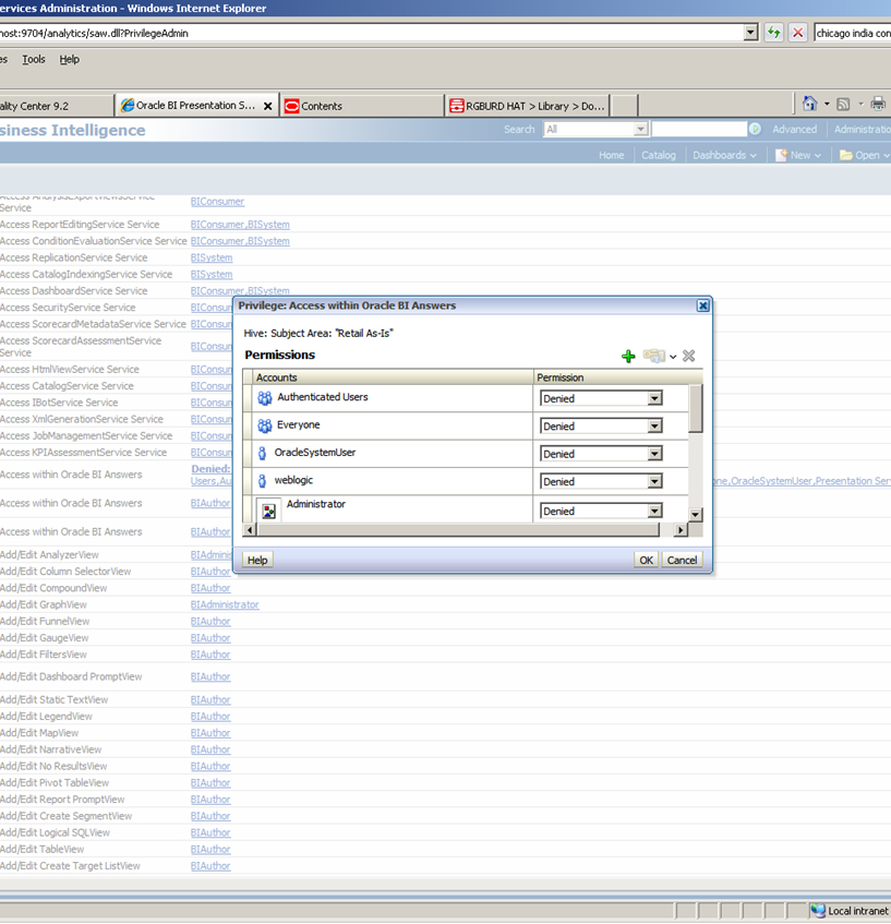
With this change, these tables can never be accessed and As-Is reporting cannot be done for inventory receipts. The same changes must be done for all the other fact areas as well. Since Retail Analytics has three subject areas (Retail As-Was, Retail As-Is and Retail Point in Time), all three are available to the user. Since As-Is components should be disabled, go to the Administration -> Manage Privileges on Oracle BI EE web and, for all the users/roles, change the permission setting to "Denied" for the As-Is subject area. This way, the As-Is subject area will not be available for reporting. The following figure displays the Administration screen.
Data Model
All the unused tables can still be in the schema and will be not used by ODI and Oracle BI EE programs. It can be maintained for future changes.
Point in Time reporting can be done with As-Was, As-Is, or with both. There are no separate ODI processes for PIT. PIT can be derived from either As-Is or As-Was data and the processing will happen during report execution. Only difference is, PIT reports cannot use aggregate tables and will always be reported from the base fact tables. There are some limitations to do this reporting in some fact areas owing to performance. For example, with the Positional facts, PIT is possible only for Product hierarchy because there are corporate aggregates for product which have the decompressed data.
The real differentiation of As-Is and As-Was in the data happens above the base fact table or when reporting is done at the parent level. Otherwise if the reporting is done at the lowest grain level, the result set will be the same for both.
In order to report Retail Analytics positional data correctly, all Retail Analytics positional compressed tables need to be seeded with source data (RMS) correctly before they can be loaded using Retail Analytics batch ETL with daily data. This seeding process is to load positional fact data for each item location combination available from RMS to Retail Analytics as initial data. This can be done by using following recommended approach. This approach assumes that user uses RMS as Retail Analytics source system and the required data are available from RMS.
This initial inventory position data loading includes loading seeding date from RMS to RA W_RTL_INV_IT_LC_DY_F, W_RTL_INV_IT_LC_WK_A, and W_RTL_INV_IT_LC_G tables. Perform the following steps:
In RMS, set the RMS vdate to the date that the seeding data will be used for.
Execute the Retail Analytics SDE script etlrefreshgensde.ksh to load RMS system data (including vdate) to the Retail Analytics temporary table RA_SRC_CURR_PARAM_G which is under Retail Analytics RMS batch user schema.
Populate the RMS IF_TRAN_DATA table with all combinations of item and location that have SOH. This can be done by using the data from the RMS ITEM_LOC_SOH table. Only columns ITEM, LOCATION, and LOC_TYPE on the IF_TRAN_DATE table will be used by the Retail Analytics SDE program and other columns on this table can be given any dummy value for this seeding purpose.
Execute the Retail Analytics SDE script invildsde.ksh to populate the Retail Analytics inventory staging table W_RTL_INV_IT_LC_DY_FS.
Make sure the Retail Analytics table W_RTL_CURR_MCAL_G has the business date and week for the current Retail Analytics business date. This is used as the date for seeding data. This date should match the RMS vdate set for the SDE program.
Execute the Retail Analytics SIL script invildsil.ksh to load the inventory seeding data from the staging table to the Retail Analytics base fact table W_RTL_INV_IT_LC_DY_F and W_RTL_INV_IT_LC_G.
Execute the Retail Analytics PLP script invildwplp.ksh to load inventory seeding data to the Retail Analytics table W_RTL_INV_IT_LC_WK_A.
Execute other inventory PLP scripts to populate the Retail Analytics inventory aggregation tables. These are chosen by the client for reporting purposes.
This initial Pricing data loading includes loading seeding date from RMS to Retail Analytics W_RTL_PRICE_IT_LC_DY_F and W_RTL_PRICE_IT_LC_G tables. Perform the following steps:
In RMS, set the RMS vdate to the date that the seeding data will be used for.
Execute the Retail Analytics SDE script etlrefreshgensde.ksh to load the RMS system data (including vdate) to the Retail Analytics temporary table RA_SRC_CURR_PARAM_G. This is under the Retail Analytics RMS batch user schema.
Modify the Retail Analytics SDE ODI program as follows:
In the ODI SDE interface SDE_RetailPriceLoad, modify the filter on PRICE_HIST table to change the filter condition from PRICE_HIST.ACTION_DATE = TO_DATE('#RA_SRC_BUSINESS_CURRENT_DT','YYYY-MM-DD') to PRICE_HIST.ACTION_DATE <= TO_DATE('#RA_SRC_BUSINESS_CURRENT_DT','YYYY-MM-DD').
Regenerate the SDE_RetailPriceFact and MASTER_ SDE_RetailPriceFact ODI scenarios.
Execute the Retail Analytics SDE script prcildsde.ksh to populate the Retail Analytics Price staging table W_RTL_PRICE_IT_LC_DY_FS.
In the Price staging table, only keep the records with the same PROD_IT_NUM, ORG_NUM, MULTI_UNIT_QYT, but maximum DAY_DT. This ensures that the staging table only contains the latest price for each combination of item, location, and multi unit quantity.
Update the Pricing staging table to replace DAY_DT with the current business date that will be used for seeding data.
Make sure the Retail Analytics table W_RTL_CURR_MCAL_G has the business date and week for the current Retail Analytics business date. This is used as the date for seeding data. This date should match RMS vdate set for the SDE program.
Execute the Retail Analytics SIL script prcilsil.ksh to load pricing seeding data from the staging table to the Retail Analytics base fact tables W_RTL_PRICE_IT_LC_DY_F and W_RTL_PRICE_IT_LC_G.
Execute the other Price PLP scripts to populate the Retail Analytics Price aggregation tables. These are chosen by the client for reporting purposes.
When the initial loading is complete, change the filter condition back and regenerate the two scenarios.
This initial Net Cost data loading includes loading seeding date from RMS to the Retail Analytics W_RTL_NCOST_IT_LC_DY_F and W_RTL_NCOST_IT_LC_G tables. Perform the following steps:
In RMS, set the RMS vdate to the date that the seeding data will be used for.
Execute the Retail Analytics SDE script etlrefreshgensde.ksh to load the RMS system data (including vdate) to the Retail Analytics temporary table RA_SRC_CURR_PARAM_G. This is under the Retail Analytics RMS batch user schema.
Modify the Retail Analytics SDE ODI program as follows:
In the ODI SDE interface SDE_RetailNetCostTempLoad, modify the filter on FUTURE_COST table to change the filter condition from FUTURE_COST.ACTIVE_DATE = to_date('#RA_SRC_BUSINESS_CURRENT_DT','YYYY-MM-DD') to FUTURE_COST.ACTIVE_DATE <= to_date('#RA_SRC_BUSINESS_CURRENT_DT','YYYY-MM-DD').
Regenerate the SDE_RETAILNETCOSTFACT and MASTER_SDE_RETAILNETCOSTFACT ODI scenarios.
Execute the Retail Analytics SDE script ncstildsde.ksh to populate the Retail Analytics Net Cost staging table W_RTL_NCOST_IT_LC_DY_FS.
In the Net Cost staging table, only keep the records with the same PROD_IT_NUM, ORG_NUM, SUPPLIER_NUM, but maximum DAY_DT. This ensures that the staging table only contains the latest net cost for each combination of item, location and supplier.
Update the Net Cost staging table to replace DAY_DT with the current business date that will be used for seeding data.
Make sure the Retail Analytics table W_RTL_CURR_MCAL_G has the business date and week for the current Retail Analytics business date. This is used as the date for seeding data. This date should match the RMS vdate set for the SDE program.
Execute the Retail Analytics SIL script ncstildsil.ksh to load Net Cost seeding data from the staging table to the Retail Analytics base fact table W_RTL_NCOST_IT_LC_DY_F and W_RTL_NCOST_IT_LC_G.
Execute other Net Cost PLP scripts to populate the Retail Analytics Net Cost aggregation tables. These are chosen by the client for reporting purpose.
When the initial loading is complete, change the filter condition back and regenerate the two scenarios.
This initial Base Cost data loading includes loading seeding date from RMS to Retail Analytics W_RTL_BCOST_IT_LC_DY_F and W_RTL_BCOST_IT_LC_G tables. Perform the following steps:
In RMS, set the RMS vdate to the date that the seeding data will be used for.
Execute the Retail Analytics SDE script etlrefreshgensde.ksh to load the RMS system data (including vdate) to the Retail Analytics temporary table RA_SRC_CURR_PARAM_G. This is under the Retail Analytics RMS batch user schema.
Modify the Retail Analytics SDE ODI program as follows:
In the ODI SDE interface SDE_RetailBaseCostTempLoad, modify the filter on the PRICE_HIST table to change the filter condition from PRICE_HIST.POST_DATE = TO_DATE('#RA_SRC_BUSINESS_CURRENT_DT','YYYY-MM-DD') to PRICE_HIST.POST_DATE <= TO_DATE('#RA_SRC_BUSINESS_CURRENT_DT','YYYY-MM-DD').
Regenerate the SDE_RETAILBASECOSTFACT and MASTER_SDE_RETAILBASECOSTFACT ODI scenarios.
Execute the Retail Analytics SDE script cstisldsde.ksh to populate the Retail Analytics Base Cost staging table W_RTL_BCOST_IT_LC_DY_FS.
In the Base Cost staging table, only keep the records with the same PROD_IT_NUM, ORG_NUM but maximum DAY_DT. This ensures that the staging table only contains the latest base cost for each combination of item and location.
Update the Base Cost staging table to replace DAY_DT with the current business date that will be used for seeding data.
Make sure the Retail Analytics table W_RTL_CURR_MCAL_G has the business date and week for the current Retail Analytics business date. This is used as the date for seeding data. This date should match the RMS vdate set for the SDE program.
Execute the Retail Analytics SIL script cstildsil.ksh to load Base Cost seeding data from staging table to the Retail Analytics base fact table W_RTL_BCOST_IT_LC_DY_F and W_RTL_BCOST_IT_LC_G.
Execute the other Base Cost PLP scripts to populate the Retail Analytics Base Cost aggregation tables. These are chosen by the client for reporting purposes.
When the initial loading is complete, change the filter condition back and regenerate the two scenarios.
Retail Analytics will extract primary image of every Item from RMS and this section provides the setup and configuration of these images in Oracle BI EE. Two scenarios are covered here based on the type of information Retail Analytics receives from RMS regarding Item Image. Retail Analytics extracts Image Name and Image Location from RMS. Image location can be a URL of a server where the images are hosted or the relative path of a shared network, which is configured in the RMS system.
Scenario 1:
In this scenario it is assumed that Retail Analytics receives URL of every item from RMS. The following items need to be configured in Oracle BI EE in order to render these Item Images.
Create an attribute in the rpd mapping to the column where URL is stored.
In answers, add this new attribute to required report. Go to the column properties of this attribute and change the data format to Image URL. Save the report.
Scenario 2:
In this scenario it is assumed that Retail Analytics does not receive URL but instead, just the location of item image as configured in RMS. The following items need to be configured in Oracle BI EE in order to render these Item Images.
Find the path, <OBIEE_INSTANCE>user_projects\domains\bifoundation_domain\servers\AdminServer\tmp\_WL_user\analytics_11.1.1
Within this directory, find the folder which has "\war\res\s_blafp" path.
Copy all the images from the RMS server to this location.
Create an attribute in the rpd mapping to the column where Item Name is mapped and drag it to the "Item As Was" and/or "Item As Is" presentation folder.
In Answers use this attribute in required reports and change the column formula as follows. '<Img src ='||'/analytics/res/s_blafp/images/'||"Item As Was"."<attribute name>"||'>' and change the data format to HTML and save the report.
Bounce all the services (including WebLogic).
Run the report to see images.