Designing Cube Metadata

This chapter provides overviews of cubes, PeopleSoft metadata, metadata types, Oracle Essbase properties, and PeopleSoft Process Scheduler Integration, and discusses how to:

• Use trees.

• Create queries.

See Also

Using PeopleSoft Tree Manager

Creating and Running Simple Queries

Understanding Cubes

The key concept of online analytical processing (OLAP) is that of a cube. In this document, we use the term cube to refer to any analytic data store. An OLAP cube is a collection of related data—a database—that has multiple dimensions. The term cube dimensions roughly describes the equivalent of fields in a relational database. In terms of data analysis, dimensions can be thought of as criteria—such as time, account, and salesperson—that can pinpoint a particular piece of data. These pieces of data are usually transactions from an online transaction processing (OLTP) system.

Although they are called cubes, OLAP databases can have more than three dimensions. In fact, most cubes have three to eight dimensions. To understand the concept of OLAP cubes, start with a simple data analysis model and then expand it.

Suppose you want to analyze unit sales of your company. You can examine the total units that were sold in a particular year, but that number might not help you understand much about your business. Instead, you might want to see unit sales broken down by time and by product. The matrix that you use to analyze this data might look like the following table, which represents a cube with two dimensions (time and product):

Dimensions and Members

In OLAP terminology, the preceding table is an OLAP cube that represents units sold dimensioned by time and product. Time and product are the dimensions of the cube, and units sold is the fact data.

In the preceding table, each dimension is subdivided into categories, called cube members, which represent individual years and products.

• In the time dimension, the members are 2001, 2002, and 2003.

• In the product dimension, the members are widgets, gadgets, doohickeys, and whatzits.

Measures and Cells

In the preceding table, the values of the most interest are not years or products. The purpose of the table is to find the number of units that were sold. Sold units make up the data element that is being evaluated or measured. In OLAP terminology, the number of units sold is called the measure, or fact, of this cube. The areas of the table where members intersect with other members represent individual measure and fact values. These intersections are called cells. The italicized cell in the preceding table represents the number of widgets sold in 2002: 6500 units.

Multiple Dimensions

The two-dimensional cube represented by the preceding table is basic for reporting purposes. For example, it does not provide data about where any of the units were sold. You can provide this information by adding another dimension, location, to the model, as shown in this diagram:

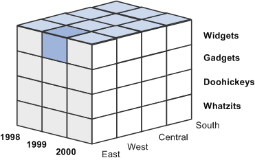
Diagram of a cube with three dimensions

The preceding three-dimensional OLAP cube represents units sold dimensioned by time, product, and location. (The location members are East, West, Central, and South.) The shaded cell represents the number of widgets sold in the East region in 1999. You could find the number of units sold for any other product in any other region at any other time by finding the cell at the intersection point of three members, one from each dimension.

Suppose you also want to factor customer accounts into the analysis. Although showing four dimensions graphically is a challenge, the result of this added dimension is clear: in our example, each cell of the OLAP cube represents the intersection of an account, a year, a region, and a product.

Hierarchy

Hierarchy is the organization of cube data elements with their reporting structures. It represents both the hierarchy and the method of consolidation in a dimension level.

The example cube has only one level in each dimension. The time dimension consists of one level containing three members (years), and the location dimension consists of one level containing four members (regions). However, the data used to build such OLAP cubes probably supports more than just one level in each dimension.

For example, when a company records a sale, that sale occurs in a particular month, which occurs in a particular quarter and in a particular year. You can examine the time dimension at one of three levels: month, quarter, or year. Likewise, you can record that each sale occurs in a particular office, in a particular city, or in a particular region. The location dimension might also have three levels, such as office, city, and region.

As mentioned, the categories found at each level of a dimension are called members. You can envision multilevel dimensions as tree diagrams, the members of which relate to each other in various parent-child relationships. Some members are parents of other members, some are children, and some are both.

This diagram shows an example of a portion of a typical time dimension with its various levels and members:

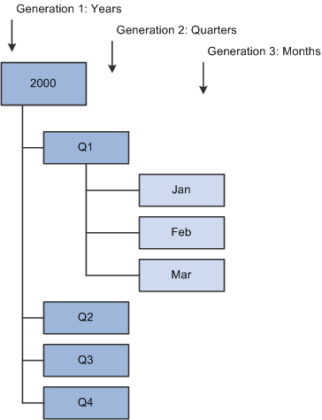
Example of a time hierarchy diagram

Each box in the diagram represents a unique member. This diagram is familiar to PeopleSoft Tree Manager users. In fact, PeopleSoft trees can play an important role in defining the hierarchy of an OLAP cube.

See Enterprise PeopleTools 8.51 PeopleBook: PeopleSoft Tree Manager.

Consolidation

Viewing the dimension of a hierarchy tells you about the organization of its members, but you should consider another facet of the dimension. You need to know how to consolidate the values that are found under child members into the value of their parent members. For example, the children might be added together to equal the parent. This scenario is certainly the case in a time dimension, in which the value for each member is added to its siblings to equal the value of its parent. (Three months can be consolidated into their parent quarter, four quarters can be consolidated into their parent year, and so on.)

This table shows the cube example, adding a second level, quarters, to the time dimension of the original example:

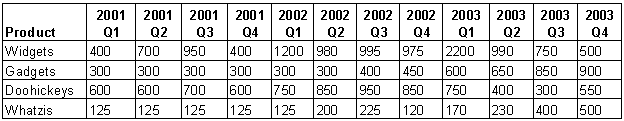
Consolidation example in tabular format

To consolidate the data at the quarterly level into the yearly level, the quarterly data is added together. The 2001 rollup is Q1 2001 + Q2 2001 + Q3 2001 + Q4 2001.

However, you also might find dimensions in which certain members are to be subtracted from their siblings, such as in a profit dimension. In such a dimension, suppose two members are at the first level, margin and total expenses, both of which are reported as positive values. To find the total profits, you would not add margin and total expenses, instead you would subtract total expenses from margin.

Understanding PeopleSoft Metadata

Metadata is data that defines data. Metadata conveys information about how data is formatted, structured, and stored. In an OLAP cube, metadata defines dimensions, levels, members, member attributes, and interrelationships of the cube. PeopleSoft Cube Manager uses two types of PeopleSoft structures, trees and queries, to define cubes.

PeopleSoft Trees

A PeopleSoft tree defines the summarization rules for a database field. It specifies, for purposes of reporting or security access, how the field values are grouped in the system.

For example, the values of the DEPTID field might identify individual departments in your organization. You could build a tree for the DEPTID field, which defines the organizational hierarchy that specifies how each department relates to the others: departments 10700 and 10800 report to the same manager, department 20200 is part of a different division, and so on.

You can easily see how you can use PeopleSoft trees to define a cube structure. Like cube dimensions, trees consist of levels and members. (In PeopleSoft Tree Manager, members are called nodes and leaves.)

See Enterprise PeopleTools 8.51 PeopleBook: PeopleSoft Tree Manager.

PeopleSoft Queries

PeopleSoft queries are SQL statements that are created by PeopleSoft Query. You can use these SELECT statements to return field values based on certain criteria. The standard PeopleSoft security mechanism can secure the data returned by PeopleSoft Query. Also, PeopleSoft Query can return data in any of the database-supported globalized formats.

You can use queries in a number of ways to define an OLAP cube. Finally, you can use queries to populate OLAP cubes with data; the query results are the rows of data that fill the cells of the cube.

See Enterprise PeopleTools 8.51 PeopleBook: PeopleSoft Query.

Understanding Metadata Types

Three types of metadata are available that define an OLAP cube:

• Dimensional metadata (hierarchy and members)

• Member property metadata (consolidation method, sign flip, and label)

• Cube metadata (dimensions and measures)

You use PeopleSoft Tree Manager and PeopleSoft Query to describe all of this metadata to PeopleSoft Cube Manager.

Understanding Oracle Essbase Properties

Oracle Essbase has the following valid property types:

• Data storage

  Data storage enables Essbase to recognize what type of storage to allocate for the member. Valid values are 0 or blank (store data), 1 (never share), 2 (label only), 3 (shared member), 4 (dynamic calculation and store), and 5 (dynamic calculation, no store).

  PeopleSoft Cube Manager sets the default value as store data for all members in the first rollup and the non-detail nodes of all other rollups. Detail nodes in secondary rollups are set to shared members.

• Expense item

  Expense item applies to account dimensions only. Essbase has certain built-in formulas that can take advantage of the knowledge that an item is an expense. To pass this knowledge on to Essbase, you should use this property. Valid values are Blank (set) and non-Blank (do not set).

• Time balance

  Time balance affects how the parent time value is calculated. Valid values are 0, 1, 2, and 3, which correspond to none, first, last, and average, respectively.

• Consolidation

  This property enables you to define the mathematical operator used for rolling up members. Most often, you expect that data is added (using the + operator) when rolled up. However, you might occasionally need to specify other operators, such as those listed in the following table:

See Also

Oracle Essbase and Cognos PowerPlay Services documentation.

Understanding PeopleSoft Process Scheduler Integration

PeopleSoft Process Scheduler includes a process type definition specifically for use with PeopleSoft Cube Builder. This process type is the Cube Builder process type, and you invoke it whenever you launch the process to create a cube from the standard run control page. During this process, the data and metadata are translated into a format that is understood by Oracle Essbase.

See Also

Defining a Cube Build Process Using Process Scheduler Manager

Using Trees

Metadata that exists in PeopleSoft trees can be particularly useful when you design cube dimensions. The main reason to use an existing tree is to leverage the rules that are associated with the outline that the tree represents. Because trees are used to validate information that is stored in the OLTP database, all of that tree information is already related to the transactional data. Using effective-dated trees in an outline generates the automatic evolution of your data that is used for data analysis.

PeopleSoft Cube Manager leverages the information that is already stored in your PeopleSoft trees as outlines upon which to build each dimension. Using the Dimension page in Essbase Cube Builder, you map a tree to a dimension so that the rollup of the resulting cube dimension is the same as that of the specified tree.

By default, data is summarized exactly as the tree is defined. Each node and detail value becomes a member of the cube hierarchy for that dimension. The descriptions of the nodes and details become the labels, or aliases, of the members.

You might want to use existing trees for your dimensions, or you might need to create new trees. If you have an existing tree that is close to what you want the dimension to look like, make a copy of the tree and modify that copy.

If the hierarchy that you want to use is a subset of an existing tree, you do not have to create a new tree. PeopleSoft Cube Builder enables you to use a subset of an existing tree by specifying a starting node, Top Node, and the number of levels below the top node of the tree to include in the hierarchy. You can use more than one tree belonging to the same business unit to define a single hierarchy.

In addition, if a tree does not provide the structure that you need for a dimension, you can add members, attributes, and generations by using one or more queries to provide the additional metadata.

PeopleSoft Cube Manager treats uppercase and lowercase characters as distinct, so the names ABC, Abc, and abc are all considered unique member names. However, Oracle Essbase offers an option to change all member names to uppercase. If you enable this option, you create problems in PeopleSoft Essbase Cube Builder with members that are identical except for their letter casing.

Note. PeopleSoft Cube Manager permits duplicate node names if you cannot avoid the duplication.

In Essbase, a dimension can have multiple rollups. The resulting total for the first rollup is calculated differently from the resulting totals for subsequent rollups. For example, a dimension exists with two rollups. Two different trees are used for these two rollups: the first tree is set up as A, B, C and the second tree is set up as A, D, C.

Assume that A, B, C, and D have the following fact data values: 2, 5, 10, and 20 respectively. The total for the first rollup, A, B, C, is 17 because the total equals 2 + 5 + 10. The total for the second rollup, A, D, C, is 10 because each parent gets its total from its children. Because C has the fact value 10, the total for C is 10. Because D is the parent of C, D gets its total from its children. Therefore, D gets 10 from C. A gets its total from its children, which is D. Therefore, A has the total value of 10.

See Also

Designing a Cube

Creating Queries

This section provides an overview of query types and discusses how to:

• Use dimension queries.

• Use data source queries.

Understanding Query Types

You can create several types of queries to use with PeopleSoft Cube Builder, all of which you must define as user (ad hoc) queries rather than role queries or database agent queries.

See Using Dimension Queries, Using Data Source Queries.

Using Dimension Queries

Dimension queries enable you to define the dimension structure using query results instead of, or in addition to, a tree. However, remember that you are using queries to create a tree-like structure.

You can convey hierarchical information by parent/child relationship or by a narrow query.

In PeopleSoft Cube Builder, dimension queries can be dynamic or static. A dynamic query indicates that any incremental change in the tables that the query uses are reflected in the next run of PS2Essbase. A static query indicates that further changes to the tables used to create the first hierarchy will not be reflected unless the hierarchy is reloaded manually.

PeopleSoft Cube Builder uses dynamic queries to populate members at the leaf levels of a hierarchy and under the same parent.

Using Data Source Queries

Data source queries define the data that you bring into the cube. Writing a data source query is straightforward; the query must return one column for each dimension and one column for the measure. Assume that you want to build a data source query for a cube containing amounts that are dimensioned by account, department, and period.

The output of your query has four columns, as shown in this table:

You can use several queries as the data source for a single cube, to load data into the measure. Every data source query that is used must include an output column for every dimension that is used and for the measure. In the version of the cube builder, only one measure is allowed per cube.

The following tables show examples of how you can use two separate queries as a data source for a cube. Note that both queries return columns for every dimension, as required, and that they differ only in which measure they include.

Results of Query 1:

Results of Query 2:

Resulting cube using Query 1 and Query 2 as data sources:

Incremental Updates

Two types of incremental updates are available:

• Metadata

  Incremental updates for metadata refers to the addition, removal, or modification of dimension members and/or their properties.

• Data

  Incremental updates for data refers to the aggregation of delta values to the cube data cells product of dimensional intersections of members.

Data Cell Types

By default, two categories of data cells are available for incremental data updates:

• Calculated data cells (or non-leaf nodes)

  Calculated data cells store values of dimensional intersections of non-level zero members (branch nodes), which are calculated based on the consolidation properties of their children.

• Stored data cells (or leaf nodes)

  The stored data cells store values of dimensional intersections of level zero members (leaves) assigned manually.

Note. You can modify the stored properties, calculated properties, or both on any member at any level.

This example shows how to create data queries for incremental updates, taking as a reference the next Accounts dimension:

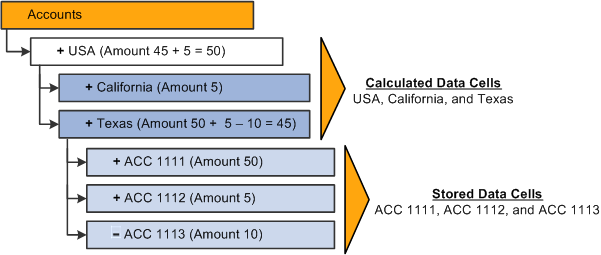
Example of how to calculate upper data cells based on stored data cells

Aggregations on Load Tool

Essbase uses the term Aggregations on Load (replace/add/subtract) as incremental updates for stored data cells. Essbase supports three data Aggregations on Load options:

• Replace current value

  Use the Replace option to overwrite or replace the currently stored value in the data cell with the value being passed. Basically, if the data file has multiple rows with the same dimensional intersection, then the last value in the data cell is stored and the previous ones are ignored.

• Add to existing values

  Use the Add option to add all the values for the stored data cell to the currently stored value. Use this option for instances in which loads are always additive, for example, an implementation that loads transactions to an already stored summary amount.

• Subtract from existing values

  Use the Subtract option as the opposite of the Add option. It subtracts the values passed from the currently stored value. This option is rarely used, but you can use it to perform an additive load that then needs to be backed out.

This example shows the aggregations on load options in the run control ID of the Create Cubes page:

Note that:

• The aggregations on load options are ignored when only metadata (dimension) is built.

• When you build multiple factories (multiple data queries) in the same build, the same Aggregations on Load option is used for all of the factories.

• The default value of the Aggregations on Load field is Replace.

• After you run the PS2Essbase process, the Aggregations on Load option serially builds each dimension and then serially builds each factory. The factory creates a data file with all the data cells to be loaded to the Essbase server.

Example: Designing Data Queries for Incremental Updates

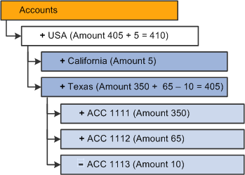
This example shows how to create data queries for each Aggregations on Load option, taking as a reference the next Accounts dimension:

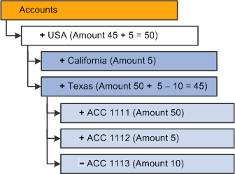
Example of how to create data queries for each Aggregations on Load option, next Accounts dimension

This example shows how to create data queries for each Aggregations on Load option, taking as a reference the next staging table that contains the data cells to be loaded:

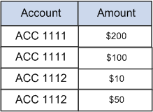
Example of how to create data queries for each Aggregations on Load option, next staging table

Essbase Cube Builder can be used to produce two different results:

1. If the Replace (replace data load) option is selected, this is the resulting dimension:

   

   Results of replacing the existing data cells

   Note. The last value passes for each cell is the valid value. In this example, cells ACC 1111 ($200) and ACC 1112 ($10) are ignored.

   When you want to perform an additive incremental update using the Replace Aggregations on Load option, you need to create a data query that summarizes repeated fields into one field. For example, to achieve an additive incremental update on stored data cells, you need to create a data query that summarizes repeated fields into one field, as in this example:

   

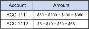
   Example of summarizing repeated fields into one field

   The SQL query is:

   

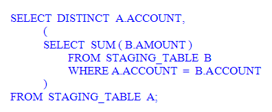
   SQL query, summarizing repeated fields into one field

   The resulting dimension is:

   

   Results of replacing incremental updates

   Note. The current stored value is overwritten and lost, therefore, in the staging table used for the data query loads, you must not eliminate the previous increments that are already loaded into Essbase. These previous increments are required to recalculate the total summarized amount in each load.
   
   In this section, the concept of staging tables is used frequently; notice that the staging tables are not tables that PeopleTools creates or maintains, the staging tables are optional customer or application tables. A staging table is any table that is used to store temporary increments to be loaded into Essbase. Depending on the option selected in the Aggregation on Load list, the staging tables may be cleaned up or maintained.

2. If the Add (addition data load) option is selected, this is the resulting dimension:

   

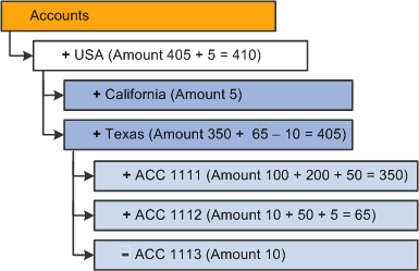
   Results of additive incremental updates: the previously stored values plus each one of the new cells that corresponds to the cube intersection are added

   Note. The resulting amounts in the dimension after the build is the same as when you want to perform an additive incremental update using the Replace Aggregations on Load option.

3. If the Subtract (subtraction data load) option is selected, this is the resulting dimension:

   

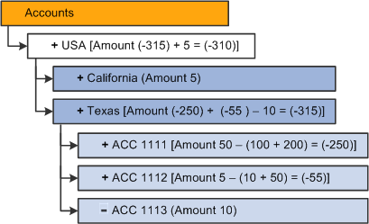
   Results of subtractive incremental updates: the previously stored values minus each one of the new cells that corresponds to the cube intersection conforms to the result for the stored data cells

In almost all instances, Replace is the preferred option over Add and Subtract because Replace makes forming queries against relational sources easier (it summarizes data to the dimensional intersection versus having duplicate rows in the load file). The Replace option is also a better alternative because it reduces the number of records to be passed to Essbase, thus improving performance. Moreover, the Add and Subtract options make the recoverability more difficult after the database fails while loading the data. Although when a recover is required, Essbase lists the number of the last rows committed in the application event log file, which is used to restart the build process.

If you run the cube using the Add or Subtract options, you need to clear the staging table after each build so that the values that are already loaded is not required again. However, PeopleSoft Cube Builder does not modify or remove the loaded cells from the staging table; either you or the application that uses the Cube Builder is responsible for cleaning up the staging table after the incremental data is loaded. If the staging table is clear, the notification of the Process Scheduler shows that the cube building process runs successfully. To successfully clear the staging table, you should create a PSJob that first runs the PS2Essbase process and then runs another AE program to clear the specific staging table.

Note. PSJob and the AE program are not provided by PeopleTools.