Generating Plans for PeopleSoft Supply Planning

This chapter provides an overview of the plan generation process and discusses how to:

• Run the Material solver.

• Run the Feasible solver.

• Run the Forecast Consumption process (SPL_FCSTCONS).

Understanding the Plan Generation Process

After you run the Load Planning Instance process (PL_LOAD_OPT) to define the planning model, you can generate a plan using the Initiate Solver component for the solver that you want to use. You can rerun any of the solvers after you have made manual changes to the plan using the Material Workbench or Capacity Workbench.

Before you generate a supply plan, ensure that you have a planning instance defined and loaded into a planning engine that you use to create the plan. Generating the plan can be an iterative process. You can run a plan multiple times to create a higher-quality plan. When you initially define the model, PeopleSoft Supply Planning passes the data that you identify as part of the planning process to the planning engine using the Load Planning Instance process. If the data is incomplete (for example, if the forecast numbers are inaccurate or if a time fence is set up improperly), stop the generation process and use the transaction system to correct incomplete or incorrect data. You can change plan data using the planning engine; however, only planned orders, order cancellations, and date changes are transferred back to the PeopleSoft transaction system.

Solvers

When you generate a material plan in PeopleSoft Supply Planning, you choose from a series of solvers. Solvers are flexible tools that analyze data and attempt to find feasible plans (based on the business planning needs) that contain no material shortages or capacity violations. Material feasibility indicates that the longest cumulative lead time exists within a manageable time frame in which no material shortages exist. Capacity feasibility indicates that no critical capacity violations exist for aggregate resources that are marked for repair in the planning time period. In addition to producing material and capacity feasible plans, solvers identify and report unavoidable instances in which the plan is jeopardized, for example, when material cannot be sourced or when insufficient lead time is available to satisfy a demand.

Using solvers, you first produce a plan based on existing supply and demand for an item to arrive at a feasible material and capacity plan. Then you manually repair infeasibilities and run more comprehensive solvers to create a plan that is ready to use when it is generated.

Time Fences

PeopleSoft Supply Planning uses fences to place boundaries on the magnitude of the planning problem, to restrict the behavior of the solvers during certain time periods, and to automate certain conditions at certain times. Solvers use fences to determine how far supply or demand tasks can be moved forward or backward to meet planning needs. You can use time fences to help determine how solvers analyze supply and demand.

Use these time fences when running PeopleSoft Supply Planning solvers:

Planning Conditions and Time Fences

Each solver processes planning conditions in conjunction with time fences. You also maintain tasks within time fences. This table lists how PeopleSoft Supply Planning solvers address planning conditions. The last column indicates whether manual rescheduling is available for the corresponding condition:

Time Buckets

Capacity plans are created in bucket sizes that are associated with each aggregate resource. Material plans that are generated by the Material solver and Feasible solver are based on time-phased netting of demands and supplies.

Item Substitution

You can predefine valid alternatives for an item when that item (the item that is used as a component in a production order) is unavailable. When using substitute items with PeopleSoft Manufacturing, PeopleSoft Supply Planning automatically suggests the substitute item when the original is in short supply or is unavailable.

You can define substitutes for an item on the Item Definition and Item Attributes by Unit pages and use them as defaults when maintaining components on a bill of material (BOM). When defining substitutes, you can specify effectivity dates and conversion factors. The conversion factor defines how many of the substitute is required to replace the original item. You can set a priority by which the substitute item with the highest priority (the substitute with the lowest priority number) is substituted first in PeopleSoft Supply Planning.

You can define general substitution options for each manufacturing business unit when you establish business unit group definitions in PeopleSoft Supply Planning.

Additionally, to enable the solvers to substitute for items, select the Allow Item Substitution option on the Initiate Feasible Solver page. When the projected quantity on hand of the primary item cannot meet the demand, the Feasible Solver can use substitutions when creating new planned production, if these criteria are met:

• You selected the Allow Item Substitution option on the business unit group definition.

• You selected options for allowing substitutions during the running of the corresponding solver.

• No partially completed operations exist for the item.

• Items have not been issued for the operation.

• Item Substitution is not frozen for the order.

  You can select the Frozen option for substitutions on the Refine Plan component for planned production orders and scheduled production orders. The mass maintenance utility also allows for component substitutions to be frozen. When a production ID or production schedule is marked as being frozen for substitutes, no substitution will be performed.

Solvers use substitutions for dependent demand only. They do not use substitutions for end items, such as sales orders, transfers, or forecasts. Solvers consider substitute items (all of the items that are effective for the period considered) according to the order of their priority.

Note. PeopleSoft Supply Planning assigns higher low-level codes to substitute items than to primary items. This ensures that primary items are planned before substitute items.

The substitute item projected quantity on hand must meet the total demand of the substitute item quantity that is needed for each primary item multiplied by the conversion factor. The solvers do not use partial substitutions. If the solvers cannot meet this demand with substitutions, they plan supply for the primary item.

Note. PeopleSoft Supply Planning solvers use valid substitutions only. However, PeopleSoft Supply Planning does not validate substitutions that are made within the transaction system and loaded into the planning instance tables.

Note. The Material solver performs substitutions only when a component is beyond its phase-out date and dependent demand exists for the component.

Production End Dates

Solvers determine the start and end dates for production by forward scheduling from the start date or backward scheduling from the due date. In most circumstances, solvers use backward scheduling; however, if not enough lead time is available for materials, or if no capacity is available and the order might be delayed, solvers use forward scheduling to find the earliest availability date for the production outputs. If a work center calendar exists for an operation, solvers validate the operation start and end dates against this calendar. If the work center calendar does not exist for an operation, PeopleSoft Supply Planning uses the business unit calendar for operation date validation.

To calculate start and end dates for production, solvers use this information:

• Operation start and operation end quantity.

• Component quantity based on the operation start quantity.

• Output quantity based on the operation end quantity.

• Effectivity dates for the components.

• Substitutions for the components.

• Offset lead time for send ahead and intransit.

• Load start offset (the duration between the operation start time and the net start time).

  Solvers calculate this number for existing production IDs.

In addition to the production start and end times, the scheduling algorithms provide the solvers with this information:

• Operation start and end time.

• Components (their required quantity and any substitutions, if checking for material capacity).

For existing production IDs and for planned production, solvers validate the operation dates against the work center or business unit calendar only.

See Also

Displaying Item Useup Information

PeopleSoft Manufacturing 9.1 PeopleBook

Common Elements Used in This Chapter

Running the Material Solver

This section provides an overview of the Material solver and discusses how to define the Material solver.

Understanding the Material Solver

The Material solver creates a simple material plan to give an accurate picture of the lead time and materials that are necessary to satisfy all of the top-level demands. It creates supplies just in time to satisfy the demand. Material planning handles supply tasks on a first-come, first-served basis. Before it creates any new planned orders, the solver reschedules nonfrozen supplies or uses existing orders. It creates new supplies only after it uses all of the existing nonfrozen supplies and the demands remain unmet. The Material solver uses existing supply or creates supply for all of the demands in the system. If the demand is beyond the phase-out date, the solver does not create new supplies for the item.

You can run the Material solver in regenerative or net change mode. In regenerative mode, the solver considers all of the items. In net change mode, the solver considers only those items with violations, items with a negative quantity at any point at or after the early fence.

This solver uses an item histogram to check for negative projected on-hand quantity at any point. A negative projected on-hand quantity can result from new demands, deleted supply, or unmet demand from the previous run. The Material solver creates planned supplies to meet negative quantity.

If lead time for a planned order pushes the start date before the early fence, the planned order will be scheduled to begin at the early fence. This may result in material shortages for both dependent and independent demands.

Additionally, the Material solver:

• Sorts all items in low-level code order.

  The Material solver solves for items in the level-code order starting with the lowest-level code. Higher assemblies have lower-level codes.

• Deletes all of the nonfrozen planned supplies for the item that is being planned

• Sorts all of the demands–sales orders, production components, transfers, forecasts and safety stock, material stock request, and end demand–by target date.

  The solver then matches supply and demand, starting with the quantity on hand. The Material solver sums all of the demands that occur at the same time.

• Sorts all of the supplies-POs, planned POs, production orders, planned production, and transfers–by date.

• Moves existing nonfrozen supplies.

• Creates supplies to meet demands.

• Cancels remaining nonfrozen supplies.

Note. The Material solver does not consider capacity.

Sourcing Options

The Material solver uses the default sourcing option only, and considers no alternate sourcing options. If the sourcing option is not effective or no default sourcing option is defined, the demands for the item are not met.

Negative Quantity On Hand

First, the Material solver satisfies negative quantity on hand, moving enough supplies to meet the negative quantity on hand. For example, it moves supplies occurring later than the early fence of the item as close to the early fence as possible, and when the total supply quantity that is moved does not satisfy the quantity on hand, it creates new supplies as close to the early fence as possible.

Fixed Periods

The Material solver includes an algorithm that determines the maximum amount that is needed between the first demand and a fixed period amount of time after all of the existing orders have been used. The fixed period is defined as a number of days on the item record. The solver consolidates demands (including safety stock) for the item for a fixed period number of days and creates a single supply.

The Material solver considers the fixed period while planning new supplies only (it does not consider the fixed period when using existing supplies). The fixed period quantity is equal to the sum of all of the demand quantities in the fixed period, plus the maximum safety limit in that period.

Page Used to Run the Material Solver

Defining Material Planning Options

Access the Material Solver page (Supply Planning, Solve Plan, Initiate Material Solver).

Run	Click to generate a material plan using the PeopleSoft Process Scheduler.
Planning Instance	Select a planning instance. Planning instances IDs define a complete set of data analyzed to create a material supply plan

Solver Settings

Plan By

Use this group box to indicate whether you want the solver to include items that have been defined in the material plan, master plan, distribution plan, or any combination. The solver includes items that are associated with the specified planned-by types only.

Select the Include Distribution Items, Include Master Items, or Include Material Items check box or any combination to items in include in the material plan.

Allow Cancellations

At the start of the solver run, the Material solver deletes planned orders that are not firm and cancels all the excess supplies at the end of the run. You can also use the check boxes in the Allow Cancellations group box to define to the Material solver which orders it can cancel when the supply is not frozen.

The system passes the frozen supply setting from the PeopleSoft Manufacturing system. You can then make the update in PeopleSoft Supply Planning and apply the update back to manufacturing. Frozen orders cannot be cancelled by the Material solver even if the orders are in excess. You can define an order as frozen using pages for each type of order. The system reschedules nonfrozen orders to meet demand on time. If the supplies are frozen and supply cannot be created on time, the system uses late frozen supply. If there is no late supply, then the supply is created in the early fence.

The default value for the check boxes is selected. Click the check box for the type of order or for the firm-planned order that you want to deselect. When you deselect an order, the system deselects the check box and does not allow the cancellation of frozen supplies. Available orders include:

Production Order: Select to allow the cancellation of production orders.

Purchase Order: Select to allow the cancellation of purchase orders.

Transfer Order: Select to allow the cancellation of transfer orders.

Firmed Planned Production: Select to allow the cancellation of firmed-firmed production. This is a production ID or production schedule that has a quantity, start date, and due date, but the bill of material and routing are frozen and the component and operation lists exist.

Firmed Planned PO: Select to allow the cancellation of firm-planned purchase orders.

Firmed Planned Transfers: Select to allow the cancellation of firm-planned transfers.

Running the Feasible Solver

This section provides an overview of the Feasible solver and discusses how to define the criteria for initiating the solver run.

Understanding the Feasible Solver

The Feasible solver is a search-based solver that uses tree-solver technology to resolve material and capacity infeasible tasks. This solver attempts material feasibility for all of the resolvable material violations between the early fence and end of time fence. If you select the Make Plan Capacity Feasible option, available on the Initiate Feasible solver page, the solver attempts capacity feasibility, as well.

Note. If you have frozen tasks, model errors, or insufficient lead time in the planning horizon, the Feasible solver may encounter capacity or material violations that cannot be resolved. In these cases, the solver identifies unavoidable problems and makes the rest of the plan feasible.

Additionally, the Feasible solver:

• Considers alternate sourcing options.

• Reschedules existing orders that are subject to capacity constraints.

• Meets demand due dates and minimizes lateness.

• Applies priority for important demands to ensure that they are met on time.

• Minimizes excess inventory.

• Generates intuitive, feasible MRP type solutions.

Solver Algorithm

When resolving material and capacity infeasible tasks, the Feasible solver deletes all of the nonfrozen planned supplies and retracts (making the supply invisible to the solver until the solver needs supply) all of the other nonfrozen supplies. This solver reschedules demand to the target date and solves for negative on-hand quantities.

Additionally, the Feasible solver sorts independent demand by demand priority, MRP level, and demand target date. Frozen demands are assumed to have the highest priority. Starting with demand that is defined with the highest priority, this solver attempts to supply all of the demand. If it is unable to find supply, it attempts to reschedule the demand for a later date. Failing that, it adds the demand to an exception list and continues to the next demand priority.

Regenerative and Net Change Run Types

When processing regenerative run types, the Feasible solver deletes all of the nonfrozen planned supplies and considers all of the other nonfrozen supply that is available for use. This solver includes frozen supply in the on-hand quantity total.

When processing net change run types, this solver considers nonfrozen supply as available for use. It includes frozen supply in the on-hand quantity total.

Lot for Lot Items

The solver maintains a pegged chain for lot-for-lot items. A lot-for-lot item is an item in which all of the sourcing options are free of order modifiers (in which supply quantities match demand quantities). When you invoke the solver, it checks any current pegging for consistency and maintains that pegging, modifying the pegging structure only when needed to make the plan material and capacity feasible.

If any supply option for an item contains an order modifier, then the solver does not consider the item a lot-for-lot item. For these items, the Feasible solver creates the pegging based on a first-in, first-out (FIFO) basis. When using the FIFO method, the solver first matches demands with the highest demand priority to the available supply.

Supply

The Feasible solver obtains supply in this order:

1. By rescheduling and using an available existing supply.

   For lot-for-lot items, this solver uses existing supply only if an exact supply and demand quantity match exists.

2. By creating new supply using the sourcing template.

   If in this process it creates new, dependant demand, it solves for this demand.

3. By using available quantity on hand when it is unable to create supply.

   For lot-for-lot items, this solver uses quantity on hand only if enough quantity on hand is available to meet the full demand quantity.

Post-Solver Phases

The Feasible solver performs these post-solver Run Lateness and Stock Phase Option processes:

• Attempts to minimize permanent excess.

• Reduces WIP and solves for safety stock.

  This phase enables the Feasible solver to maintain the feasibility of the schedule, while searching for opportunities to reduce excess inventory that occurs between the early fence and end of time fence, and to search for opportunities to satisfy unfulfilled safety-stock requirements.

• Performs lateness reduction phase.

  This phase maintains the feasibility of the schedule while searching for opportunities to reduce the lateness of demands that have been delayed past their due date. These opportunities can exist due to gaps left behind in capacity or when alternate build options are defined in the model using different bills of material.

Late Supply Calculations

When the Feasible Solver cannot supply on-time quantities for top-level demand which is ordered by demand priority, item low-level code and due date and time, it:

1. Attempts to use available planned on-hand quantity that's not allocated to other demand or safety stock.

2. For the remaining demand quantity that's not covered by the first step, attempts to use existing supplies including purchase orders, production process IDs, and transfers.

   The order in which the solver selects the supplies is based on the current planned due date and time of the orders. If the selected purchase order, production process, or transfer has a start date and time after the early fence and if the supply is late for the demand, the solver attempts to reschedule it to start at the early fence. The system does not reschedule supplies that start at or before the early fence.

   If a transfer order or a production order is selected, the solver checks the order's demand. The solver first attempts to use the available planned on hand quantity, similar to the process described in step 1, to cover the dependent demand. Then, the solver attempts to use existing purchase orders for the demand, similar to the process described in step 2, but the solver does not use existing production ID or transfer supplies. If there is still remaining demand quantity, the solver attempts to create planned supplies using default sourcing options described in step 4.

3. If there is still remaining demand quantity not covered by step 2, you can select the Transfer Network Onhand check box in the Feasible Solver to indicate that you want to create planned transfers.

   Using this functionality, the system creates planned transfers for each transfer option on the sourcing template, ordered by sourcing template priority. The planned transfer is created with the available planned on hand quantity if there are any from the source business unit, starting at the early fence of the source business unit and item. If the available on hand at the source business unit is more than the demand quantity, the solver transfers up to the demand quantity. If the supply is not enough to cover the demand, the solver continues to the next transfer option on the sourcing template until the demand quantity is fully covered or all transfer options are exhausted.

4. If there are still remaining demand quantity after step 3, the solver attempts to create planned supplies using the default sourcing option.

   If there is dependent demand created, such as in the case of planned transfer or production, the solver explodes down each level of the supply chain. For each lower-level dependent demand the solver attempts to use available planned on hand quantity first, then it attempts to use existing purchase orders similar to process described in step 2, but the solver does not use existing production process ID or transfer supplies. If the dependent demand quantity is still not satisfied, the solver creates planned supplies using the default sourcing option.

5. Finishes the first top-level demand and advances to the next demand by repeating steps 1 to 4.

Page Used to Run the Feasible Solver

Defining Criteria for the Feasible Solver

Access the Feasible Solver page (Supply Planning, Solve Plan, Initiate Feasible Solver).

Solver Settings

Feasibility Options

Allow Cancellations

At the start of the solver run, the Feasible solver deletes planned orders that are not firm and cancels all the excess supplies at the end of the run. You can use the check boxes in the Allow Cancellations group box to define to the feasible solver which orders it can cancel.

The system passes the frozen supply setting from the PeopleSoft Manufacturing system. You can then make the update in PeopleSoft Supply Planning and apply the update back to manufacturing.

The default value for the check boxes is selected. Click the check box for the type of order or for the firm-planned order that you want to deselect. When you deselect an order, the system deselects the check box and does not allow the cancellation of frozen supplies.

The default value for the check boxes is selected. Click the check box for the type of order or for the firm-planned order that you want to deselect. When you deselect an order, the system deselectss the check box and does not allow the cancellation. Available orders include:

Production Order: Select to allow the cancellation of production orders.

Purchase Order: Select to allow the cancellation of purchase orders.

Transfer Order: Select to allow the cancellation of transfer orders.

Firmed Planned Production: Select to allow the cancellation of firmed-firmed production. This is a production ID or production schedule that has a quantity, start date, and due date, but the bill of material and routing are frozen and the component and operation lists exist.

Firmed Planned PO: Select to allow the cancellation of firm-planned purchase orders.

Firmed Planned Transfers: Select to allow the cancellation of firm-planned transfers.

Running the Forecast Consumption Process

This section provides overviews of forecast consumption, data extract methods, and forecast allocation and lists the page that is used to run the Forecast Consumption process.

Understanding Forecast Consumption

When you create a planning instance, you determine the forecast origins and types that you allocate and consume. The forecast consumption process uses these forecast specifications that you set up during the planning instance creation. Forecast consumption and allocation can consist of as many as four phases. The forecast options that you defined when you set up the planning instance determine order availability and carrying out of these phases. The phases are:

1. Allocation from external time periods into PeopleSoft Supply Planning forecasting time periods.

2. Forecast consumption with actual demands to create a net forecast.

3. Net forecast adjustment to account for deviations of actual demand from forecasted demand.

4. Net forecast breakdown to reduce a large forecast into smaller, more manageable portions.

This table lists the order of these phases when you source forecasts from PeopleSoft Inventory:

This table describes the order of these phases when you source forecasts from PeopleSoft Publish Forecast tables that use forecast from Demantra Demand Management:

Understanding Data Extract Methods

This diagram illustrates how PeopleSoft Supply Planning extracts forecast data from demand management and inventory transaction systems:

Extracting forecast data from transaction systems

When PeopleSoft Supply Planning completes the initial data extraction, it writes the only bucketed unconsumed forecasts for PeopleSoft Inventory items to the Unconsumed Forecast table (PL_FORECAST_UNC). You can maintain the forecast quantities and daily weights for this forecast under the Refine Plan - Forecasting menu.

This diagram illustrates different scenarios for processing forecasts in PeopleSoft Supply Planning:

Processing forecasts in PeopleSoft Supply Planning

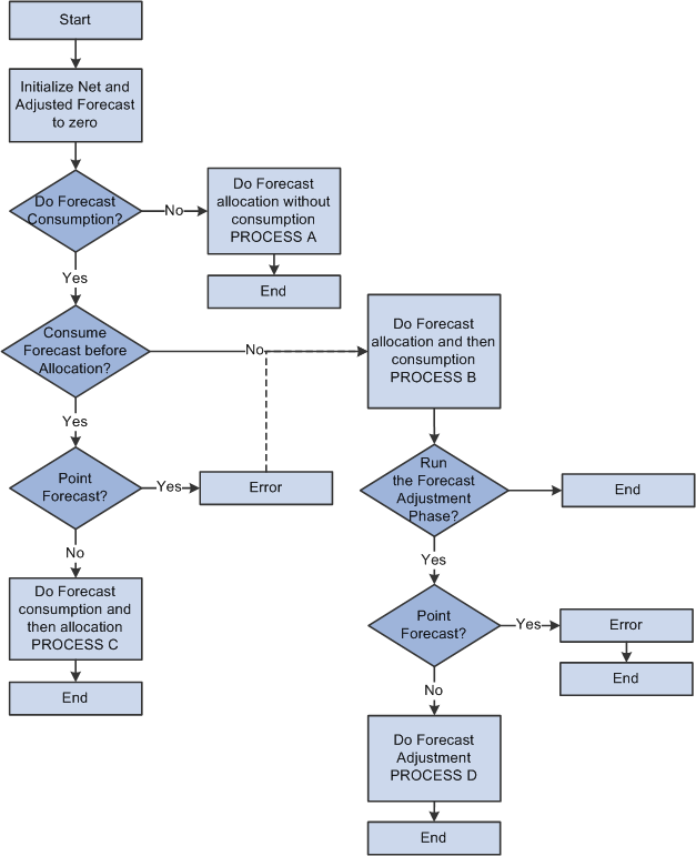
Forecast Allocation Without Consumption (Process A)

If you define a run control to indicate that you do not require forecast consumption, PeopleSoft Supply Planning assumes that the entered forecasts are net forecasts and performs these steps:

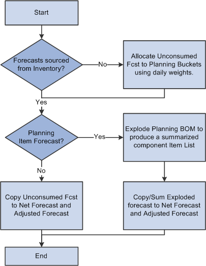
Forecast allocation without consumption

PeopleSoft Supply Planning performs these steps for each item in the Unconsumed Forecast table (PL_FORECAST_UNC).

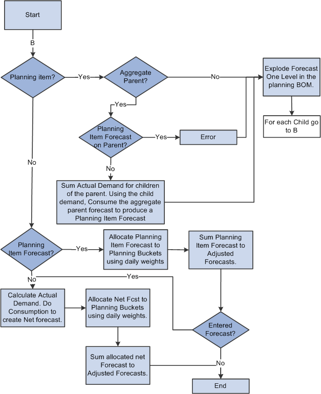
Forecast Allocation Followed by Forecast Consumption (Process B)

In this scenario, PeopleSoft Supply Planning converts forecasts from PeopleSoft Publish Forecast table buckets into PeopleSoft Supply Planning buckets, and then consumes the forecast:

Forecast allocation followed by forecast consumption

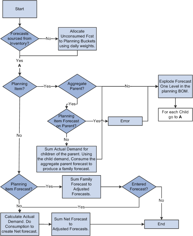
Forecast Consumption Followed by Forecast Allocation (Process C)

In this scenario, PeopleSoft Supply Planning consumes a forecast using period buckets, producing a net forecast for each PeopleSoft Publish Forecast table. PeopleSoft Supply Planning then allocates the net forecast into planning periods.

Forecast consumption followed by forecast allocation

Forecast Adjustment

PeopleSoft Supply Planning adjusts forecast planning bucket quantities to match known actual demand. Using a process called forecast adjustment, PeopleSoft Supply Planning moves an unconsumed forecast that exists before the demand fence, prorating the unconsumed forecast to periods after the demand fence. Forecast adjustment is necessary when the PeopleSoft Publish Forecast table and the bucket size is large (monthly or greater) and the PeopleSoft Supply Planning bucket size is small (for example, weekly).

PeopleSoft Supply Planning adjusts forecast when:

• PeopleSoft Publish Forecast tables provide unconsumed bucketed forecasts for PeopleSoft Supply Planning. This forecast data comes from Demantra Demand Management.

• You enable forecast consumption (select Allow Forecast Consumption on the Load Planning Instance - Orders/Forecast: Forecast page).

• Consumption occurs after the allocation from PeopleSoft Publish Forecast table buckets to PeopleSoft Supply Planning buckets.

PeopleSoft Supply Planning considers only whole PeopleSoft Supply Planning buckets that occur before the demand data and that fit into the PeopleSoft Publish Forecast table bucket for the unconsumed forecast. PeopleSoft Supply Planning distributes an unconsumed forecast evenly across the remaining planning buckets that match the demand management period.

Understanding Forecast Allocation

PeopleSoft Supply Planning enables you to control how you allocate forecasts from PeopleSoft Publish Forecast table periods into PeopleSoft Supply Planning forecast buckets.

PeopleSoft Supply Planning breaks down PeopleSoft Publish Forecast table bucket forecasts into daily forecasts using the PeopleSoft daily weights, then aggregates the daily forecasts into planning buckets.

See Setting Up Calendar and Weight Profiles.

Example: Forecast Allocation

In this example, PeopleSoft Supply Planning allocates these raw PeopleSoft Publish Forecast tables unconsumed forecasts:

Assume that these daily weights exist and are applied in PeopleSoft Publish Forecast tables for all three months:

PeopleSoft Supply Planning forecast buckets are weekly and always begin on a Sunday. The plan starts on Monday, January 21. This table lists how PeopleSoft Supply Planning allocates the forecast:

Page Used to Run the Forecast Consumption Process