9 Built-In Aggregate Functions
This chapter provides a reference to built-in aggregate functions included in Oracle Continuous Query Language (Oracle CQL). Built-in aggregate functions perform a summary operation on all the values that a query returns.
For more information, see Section 1.1.11, "Functions".
This chapter includes the following section:
9.1 Introduction to Oracle CQL Built-In Aggregate Functions
Table 9-1 lists the built-in aggregate functions that Oracle CQL provides:
Table 9-1 Oracle CQL Built-in Aggregate Functions
| Type | Function |
|---|---|
|
Aggregate |
|
|
Aggregate (incremental computation) |
|
|
Extended aggregate |
Specify distinct if you want Oracle Event Processing to return only one copy of each set of duplicate tuples selected. Duplicate tuples are those with matching values for each expression in the select list. For more information, see aggr_distinct_expr.
Oracle Event Processing does not support nested aggregations.
Note:
Built-in function names are case sensitive and you must use them in the case shown (in lower case).
Note:
In stream input examples, lines beginning with h (such as h 3800) are heartbeat input tuples. These inform Oracle Event Processing that no further input will have a timestamp lesser than the heartbeat value.
For more information, see:
9.1.1 Built-In Aggregate Functions and the Where, Group By, and Having Clauses
In Oracle CQL, the where clause is applied before the group by and having clauses. This means the Oracle CQL statement in Example 9-1 is invalid:
Example 9-1 Invalid Use of count
<query id="q1"><![CDATA[
    select * from InputChanel[rows 4 slide 4] as ic where count(*) = 4
]]></query>
Instead, you must use the Oracle CQL statement that Example 9-2 shows:
Example 9-2 Valid Use of count
<query id="q1"><![CDATA[
    select * from InputChanel[rows 4 slide 4] as ic, count(*) as myCount having myCount = 4
]]></query>
For more information, see:
avg

avg returns average value of expr.
This function takes as an argument any bigint, float, or int datatype. The function returns a float regardless of the numeric datatype of the argument.
Consider the query float_avg in Example 9-3 and the data stream S3 in Example 9-4. Stream S3 has schema (c1 float). The query returns the relation in Example 9-5. Note that the avg function returns a result of NaN if the average value is not a number. For more information, see Section 2.3.2, "Numeric Literals".
Example 9-3 avg Function Query
<query id="float_avg"><![CDATA[
    select avg(c1) from S3[range 5]
]]></query>
count

(arith_expr::=, attr::=, identifier::=)
count returns the number of tuples returned by the query as an int value.
The return value depends on the argument as Table 9-2 shows.
Table 9-2 Return Values for COUNT Aggregate Function
| Input Argument | Return Value |
|---|---|
|
|
The number of tuples where |
|
|
The number of all tuples, including duplicates and nulls. |
|
|
The number of all tuples that match the correlation variable |
|
|
The number of tuples that match correlation variable |
count never returns null.
Consider the query q2 in Example 9-6 and the data stream S2 in Example 9-7. Stream S2 has schema (c1 integer, c2 integer). The query returns the relation in Example 9-8.
Example 9-6 count Function Query
<query id="q2"><![CDATA[
    SELECT COUNT(c2), COUNT(*) FROM  S [RANGE 10]
]]></query>
Example 9-8 count Function Relation Output
Timestamp                Tuple Kind  Tuple
-9223372036854775808:    +           0,0
1000:                    -           0,0
1000:                    +           1,1
2000:                    -           1,1
2000:                    +           1,2
3000:                    -           1,2
3000:                    +           2,3
6000:                    -           2,3
For more information, see:
first
first returns the value of the specified stream element the first time the specified pattern is matched.
The type of the specified stream element may be any of:
-
bigint -
integer -
byte -
char -
float -
interval -
timestamp
The return type of this function depends on the type of the specified stream element.
This function takes a single argument made up of the following period-separated values:
-
identifier1: the name of a pattern as specified in aDEFINEclause. -
identifier2: the name of a stream element as specified in aCREATE STREAMstatement.
See Also:
Consider the query q9 in Example 9-9 and the data stream S0 in Example 9-10. Stream S0 has schema (c1 integer, c2 float). This example defines pattern C as C.c1 = 7. It defines firstc as first(C.c2). In other words, firstc will equal the value of c2 the first time c1 = 7. The query returns the relation in Example 9-11.
Example 9-9 first Function Query
<query id="q9"><![CDATA[
    select
        T.firstc,
        T.lastc,
        T.Ac1,
        T.Bc1,
        T.avgCc1,
        T.Dc1
    from
        S0
    MATCH_RECOGNIZE (
        MEASURES
            first(C.c2) as firstc,
            last(C.c2) as lastc,
            avg(C.c1) as avgCc1,
            A.c1 as Ac1,
            B.c1 as Bc1,
            D.c1 as Dc1
        PATTERN(A B C* D)
        DEFINE
            A as A.c1 = 30,
            B as B.c2 = 10.0,
            C as C.c1 = 7,
            D as D.c1 = 40
    ) as T
]]></query>
last
last returns the value of the specified stream element the last time the specified pattern is matched.
The type of the specified stream element may be any of:
-
bigint -
integer -
byte -
char -
float -
interval -
timestamp
The return type of this function depends on the type of the specified stream element.
This function takes a single argument made up of the following period-separated values:
-
identifier1: the name of a pattern as specified in aDEFINEclause. -
identifier2: the name of a stream element as specified in aCREATE STREAMstatement.
See Also:
Consider the query q9 in Example 9-12 and the data stream S0 in Example 9-13. Stream S1 has schema (c1 integer, c2 float). This example defines pattern C as C.c1 = 7. It defines lastc as last(C.c2). In other words, lastc will equal the value of c2 the last time c1 = 7. The query returns the relation in Example 9-14.
Example 9-12 last Function Query
<query id="q9"><![CDATA[
    select
        T.firstc,
        T.lastc,
        T.Ac1,
        T.Bc1,
        T.avgCc1,
        T.Dc1
    from
        S0
    MATCH_RECOGNIZE (
        MEASURES
            first(C.c2) as firstc,
            last(C.c2) as lastc,
            avg(C.c1) as avgCc1,
            A.c1 as Ac1,
            B.c1 as Bc1,
            D.c1 as Dc1
        PATTERN(A B C* D)
        DEFINE
            A as A.c1 = 30,
            B as B.c2 = 10.0,
            C as C.c1 = 7,
            D as D.c1 = 40
    ) as T
]]></query>
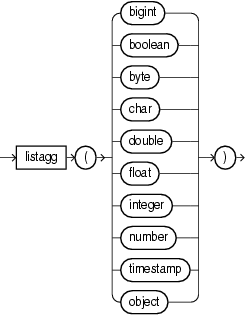
listagg

listagg returns a java.util.List containing the Java equivalent of the function's argument.
Note that when a user-defined class is used as the function argument, the class must implement the equals method.
In Example 9-15, "listagg Query", view v1 aggregates the values from the third column of Example 9-16, "listagg Example Input" into a java.util.List (the default return type) and a java.util.LinkedHashSet. Query q1 then selects the size of each to generate the output in Example 9-17, "listagg Relation Output".
<view id="v1"><![CDATA[
    ISTREAM(select c1, listAgg(c3) as l1,
        java.util.LinkedHashSet(listAgg(c3)) as set1
    from S1
    group by c1)
]]></view>

<query id="q1"><![CDATA[
    select v1.l1.size(), v1.set1.size()
    from v1
]]></query>
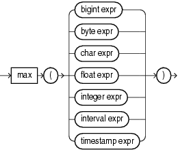
max

max returns maximum value of expr. Its datatype depends on the datatype of the argument.
Consider the query test_max_timestamp in Example 9-18 and the data stream S15 in Example 9-19. Stream S15 has schema (c1 int, c2 timestamp). The query returns the relation in Example 9-20.
Example 9-18 max Function Query
<query id="test_max_timestamp"><![CDATA[
    select max(c2) from S15[range 2]
]]></query>
Example 9-19 max Function Stream Input
Timestamp   Tuple
  10        1,"08/07/2004 11:13:48"
2000         ,"08/07/2005 11:13:48"
3400        3,"08/07/2006 11:13:48"
4700         ,"08/07/2007 11:13:48"
h 8000
h 200000000
Example 9-20 max Function Relation Output
Timestamp   Tuple Kind  Tuple
   0:       +
  10:       -
  10:       +           08/07/2004 11:13:48
2000:       -           08/07/2004 11:13:48
2000:       +           08/07/2005 11:13:48
2010:       -           08/07/2005 11:13:48
2010:       +           08/07/2005 11:13:48
3400:       -           08/07/2005 11:13:48
3400:       +           08/07/2006 11:13:48
4000:       -           08/07/2006 11:13:48
4000:       +           08/07/2006 11:13:48
4700:       -           08/07/2006 11:13:48
4700:       +           08/07/2007 11:13:48
5400:       -           08/07/2007 11:13:48
5400:       +           08/07/2007 11:13:48
6700:       -           08/07/2007 11:13:48
6700:       +
min

min returns minimum value of expr. Its datatype depends on the datatype of its argument.
Consider the query test_min_timestamp in Example 9-21 and the data stream S15 in Example 9-22. Stream S15 has schema (c1 int, c2 timestamp). The query returns the relation in Example 9-23.
Example 9-21 min Function Query
<query id="test_min_timestamp"><![CDATA[
    select min(c2) from S15[range 2]
]]></query>
Example 9-22 min Function Stream Input
Timestamp   Tuple
  10        1,"08/07/2004 11:13:48"
2000         ,"08/07/2005 11:13:48"
3400        3,"08/07/2006 11:13:48"
4700         ,"08/07/2007 11:13:48"
h 8000
h 200000000
Example 9-23 min Function Relation Output
Timestamp   Tuple Kind  Tuple
   0:       +
  10:       -
  10:       +           08/07/2004 11:13:48
2000:       -           08/07/2004 11:13:48
2000:       +           08/07/2004 11:13:48
2010:       -           08/07/2004 11:13:48
2010:       +           08/07/2005 11:13:48
3400:       -           08/07/2005 11:13:48
3400:       +           08/07/2005 11:13:48
4000:       -           08/07/2005 11:13:48
4000:       +           08/07/2006 11:13:48
4700:       -           08/07/2006 11:13:48
4700:       +           08/07/2006 11:13:48
5400:       -           08/07/2006 11:13:48
5400:       +           08/07/2007 11:13:48
6700:       -           08/07/2007 11:13:48
6700:       +
sum

sum returns the sum of values of expr. This function takes as an argument any bigint, float, or integer expression. The function returns the same datatype as the numeric datatype of the argument.
Consider the query q3 in Example 9-24 and the data stream S1 in Example 9-25. Stream S1 has schema (c1 integer, c2 bigint). The query returns the relation in Example 9-26. For more information on range, see "Range-Based Stream-to-Relation Window Operators".
Timestamp   Tuple
1000         5,
1000        10,5
2000          ,4
3000        30,6
5000        45,44
7000        55,3
h 200000000
xmlagg
xmlagg returns a collection of XML fragments as an aggregated XML document. Arguments that return null are dropped from the result.
You can control the order of fragments using an ORDER BY clause. For more information, see Section 20.2.9, "Sorting Query Results".
This section describes the following xmlagg examples:
xmlagg Function and the xmlelement Function
Consider the query tkdata67_q1 in Example 9-27 and the input relation in Example 9-28. Stream tkdata67_S0 has schema (c1 integer, c2 float). This query uses xmlelement to create XML fragments from stream elements and then uses xmlagg to aggregate these XML fragments into an XML document. The query returns the relation in Example 9-29.
For more information about xmlelement, see "xmlelement_expr".
<query id="tkdata67_q1"><![CDATA[
    select
        c1,
        xmlagg(xmlelement("c2",c2))
    from
        tkdata67_S0[rows 10]
    group by c1
]]></query>
Example 9-28 xmlagg Relation Input
Timestamp           Tuple
 1000               15, 0.1
 1000               20, 0.14
 1000               15, 0.2
 4000               20, 0.3
10000               15, 0.04
h 12000
Example 9-29 xmlagg Relation Output
Timestamp   Tuple Kind  Tuple
1000:       +           15,<c2>0.1</c2>
                           <c2>0.2</c2>
1000:       +           20,<c2>0.14</c2>
4000:       -           20,<c2>0.14</c2>
4000:       +           20,<c2>0.14</c2>
                           <c2>0.3</c2>
10000:      -           15,<c2>0.1</c2>
                           <c2>0.2</c2>
10000:      +           15,<c2>0.1</c2>
                           <c2>0.2</c2>
                           <c2>0.04</c2>
xmlagg Function and the ORDER BY Clause
Consider the query tkxmlAgg_q5 in Example 9-30 and the input relation in Example 9-31. Stream tkxmlAgg_S1 has schema (c1 int, c2 xmltype). These query selects xmltype stream elements and uses XMLAGG to aggregate them into an XML document. This query uses an ORDER BY clause to order XML fragments. The query returns the relation in Example 9-32.
Example 9-30 xmlagg and ORDER BY Query
<query id="tkxmlAgg_q5"><![CDATA[
    select
        xmlagg(c2),
        xmlagg(c2 order by c1)
    from
        tkxmlAgg_S1[range 2]
]]></query>
Example 9-31 xmlagg and ORDER BY Relation Input
Timestamp           Tuple
1000                1, "<a>hello</a>"
2000               10, "<b>hello1</b>"
3000               15, "<PDRecord><PDName>hello</PDName></PDRecord>"
4000                5, "<PDRecord><PDName>hello</PDName><PDName>hello1</PDName></PDRecord>"
5000               51, "<PDRecord><PDId>6</PDId><PDName>hello1</PDName></PDRecord>"
6000               15, "<PDRecord><PDId>46</PDId><PDName>hello2</PDName></PDRecord>"
7000               55, "<PDRecord><PDId>6</PDId><PDName>hello2</PDName><PDName>hello3</PDName></PDRecord>"
Example 9-32 xmlagg and ORDER BY Relation Output
Timestamp   Tuple Kind  Tuple
    0:      +
1000:       -
1000:       +           <a>hello</a>
                       ,<a>hello</a>
2000:       -           <a>hello</a>
                       ,<a>hello</a>
2000:       +           <a>hello</a>
                        <b>hello1</b>
                       ,<a>hello</a>
                        <b>hello1</b>
3000:       -           <a>hello</a>
                        <b>hello1</b>
                       ,<a>hello</a>
                        <b>hello1</b>
3000:       +           <b>hello1</b>
                        <PDRecord>
                          <PDName>hello</PDName>
                        </PDRecord>
                       ,<b>hello1</b>
                        <PDRecord>
                          <PDName>hello</PDName>
                        </PDRecord>
4000:       -           <b>hello1</b>
                        <PDRecord>
                          <PDName>hello</PDName>
                        </PDRecord>
                       ,<b>hello1</b>
                        <PDRecord>
                          <PDName>hello</PDName>
                        </PDRecord>
4000:       +           <PDRecord>
                          <PDName>hello</PDName>
                        </PDRecord>
                        <PDRecord>
                          <PDName>hello</PDName>
                          <PDName>hello1</PDName>
                        </PDRecord>
                       ,<PDRecord>
                          <PDName>hello</PDName>
                          <PDName>hello1</PDName>
                        </PDRecord>
                        <PDRecord>
                          <PDName>hello</PDName>
                        </PDRecord>
5000:       -           <PDRecord>
                          <PDName>hello</PDName>
                        </PDRecord>
                        <PDRecord>
                          <PDName>hello</PDName>
                          <PDName>hello1</PDName>
                        </PDRecord>
                       ,<PDRecord>
                          <PDName>hello</PDName>
                          <PDName>hello1</PDName>
                        </PDRecord>
                        <PDRecord>
                          <PDName>hello</PDName>
                        </PDRecord>
5000:       +           <PDRecord>
                          <PDName>hello</PDName>
                          <PDName>hello1</PDName>
                        </PDRecord>
                        <PDRecord>
                          <PDId>6</PDId>
                          <PDName>hello1</PDName>
                        </PDRecord>
                       ,<PDRecord>
                          <PDName>hello</PDName>
                          <PDName>hello1</PDName>
                        </PDRecord>
                        <PDRecord>
                          <PDId>6</PDId>
                          <PDName>hello1</PDName>
                        </PDRecord>
6000:       -           <PDRecord>
                          <PDName>hello</PDName>
                          <PDName>hello1</PDName>
                        </PDRecord>
                        <PDRecord>
                          <PDId>6</PDId>
                          <PDName>hello1</PDName>
                        </PDRecord>
                       ,<PDRecord>
                          <PDName>hello</PDName>
                          <PDName>hello1</PDName>
                        </PDRecord>
                        <PDRecord>
                          <PDId>6</PDId>
                          <PDName>hello1</PDName>
                        </PDRecord>
6000:       +           <PDRecord>
                          <PDId>6</PDId>
                          <PDName>hello1</PDName>
                        </PDRecord>
                        <PDRecord>
                          <PDId>46</PDId>
                          <PDName>hello2</PDName>
                        </PDRecord>
                       ,<PDRecord>
                          <PDId>46</PDId>
                          <PDName>hello2</PDName>
                        </PDRecord>
                        <PDRecord>
                          <PDId>6</PDId>
                          <PDName>hello1</PDName>
                        </PDRecord>
7000:       -           <PDRecord>
                          <PDId>6</PDId>
                          <PDName>hello1</PDName>
                        </PDRecord>
                        <PDRecord>
                          <PDId>46</PDId>
                          <PDName>hello2</PDName>
                        </PDRecord>
                       ,<PDRecord>
                          <PDId>46</PDId>
                          <PDName>hello2</PDName>
                        </PDRecord>
                        <PDRecord>
                          <PDId>6</PDId>
                          <PDName>hello1</PDName>
                        </PDRecord>